Part 5: LLM Foundations — transformers, RLHF, sampling

Last update: July 2026. All opinions are my own.

GenAI Engineering — Interview Prep · Part 5/15

This is the foundational post of the interview-prep series. If you're preparing for an AI Engineer or Generative AI role, the interviewer will almost always open here — with "so, what is a large language model?" and drill down from transformers to sampling to alignment. This post walks the whole surface once, slowly, with the diagrams that make each concept click.

Why the interviewer will start here

Every GenAI interview I've seen (and I've been through a few by now) opens with a version of the same question. Tell me about how a modern LLM works. Or walk me through what happens after pretraining. Or if I turn temperature to zero, what changes?

The interviewer isn't looking for a memorised paragraph. They're looking for how many levels deep you can go before you flinch. You need to be able to move fluidly from "an LLM predicts the next token" down to "self-attention is a weighted average where the weights come from softmax over query-key dot products divided by root d_k" — and back up again. Both directions.

So the goal of this post isn't to be exhaustive. It's to make sure that when the interviewer taps on any one of these concepts, you have the mental picture already loaded. What it is, why it matters, how it works, and the interview trap to avoid. Nine concepts, one at a time, in the order they build on each other.

1. What is a Large Language Model

An LLM is a neural network — almost always a transformer decoder — trained to predict the next token in a sequence. That's the entire objective. Given "The cat sat on the", predict "mat". Do that on a few trillion tokens of internet text, and the network is forced to encode syntax, semantics, world knowledge, style, and code into its parameters as a side effect of getting the next token right.

The "large" part is the interesting bit. Modern LLMs have somewhere between $10^9$ and $10^{12}$ parameters, are trained on $10^{12}$ to $10^{13}$ tokens, and cost $10^{23}$ to $10^{25}$ floating-point operations to train. Somewhere around a few billion parameters, something strange starts happening — the model develops abilities that smaller models simply don't have. Translation, arithmetic, code, following instructions in natural language. Nobody explicitly trained it to do any of that. We'll come back to this under scaling laws.

Interview angle. If they ask "what is an LLM?", don't just say "it predicts the next word." Say it predicts the next token, mention the scale (parameters, tokens, compute), and mention that most modern LLMs are decoder-only transformers trained autoregressively. That last sentence signals you know the architecture matters — encoder-only (BERT), decoder-only (GPT), and encoder-decoder (T5, original transformer) are three different beasts. Modern chat models are almost all decoder-only.

2. Transformer architecture and self-attention

This is the section they will spend the most time on. If you nail the transformer, you've bought yourself a lot of goodwill for the rest of the interview.

The transformer was introduced in Vaswani et al. 2017, "Attention is All You Need". Before that, sequence models were RNNs and LSTMs — they processed tokens one at a time, which was slow and struggled with long-range dependencies. The transformer replaced recurrence with self-attention, which lets every token look at every other token in parallel.

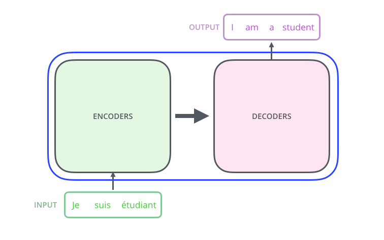
Transformer as a stack of encoders and decoders, from Jay Alammar's Illustrated Transformer

The classic view: a stack of encoders on the left feeding a stack of decoders on the right. Modern chat LLMs (GPT, Claude, Llama) drop the encoder and use only the decoder stack. Source: Jay Alammar — The Illustrated Transformer.

Self-attention: the math

Every token in the input becomes three vectors: a Query $Q$ , a Key $K$ , and a Value $V$ . You get them by multiplying the token's embedding by three learned matrices $W_Q$ , $W_K$ , $W_V$ . That's it — three linear projections.

Then you compute attention with the formula everyone will ask you to write on the whiteboard:

\text{Attention}(Q, K, V) = \text{softmax}\left(\frac{Q K^T}{\sqrt{d_k}}\right) V

Piece by piece:

$Q K^T$ — every query dotted with every key. This gives a matrix of "how much should token $i$ care about token $j$ ?" scores.
$\sqrt{d_k}$ — divide by the square root of the key dimension. Without this, the dot products get big, the softmax saturates, gradients die. This is the "scaled" in scaled dot-product attention.
$\text{softmax}(...)$ — turn scores into a probability distribution across all tokens. Now each row sums to 1.
Multiply by $V$ — take a weighted average of the value vectors, using those attention weights. The output for token $i$ is a blend of all other tokens' values, weighted by how relevant they are to $i$ .

Self-attention Q, K, V vectors from Jay Alammar's Illustrated Transformer

Each input embedding produces three vectors — Query, Key, Value — via three learned weight matrices. Source: Jay Alammar — The Illustrated Transformer.

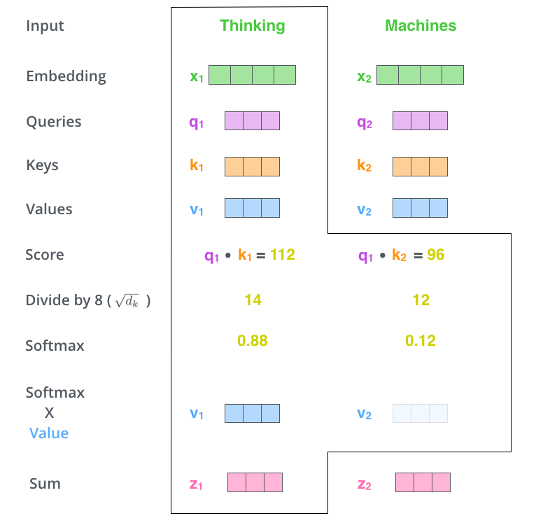
Full self-attention computation producing the output vector

The full computation: score, scale, softmax, weighted sum of values. This is what runs for every token, in parallel.

Multi-head attention

One attention head learns one type of relationship — maybe syntactic, maybe co-reference. Multi-head attention runs $h$ heads in parallel with separate $W_Q$ , $W_K$ , $W_V$ matrices, then concatenates the outputs and projects them back down. Each head is free to specialise. GPT-3 used 96 heads. Empirically, some heads track subjects and verbs, some track names, some track punctuation. You never tell them what to specialise in — they self-organise from the pretraining objective.

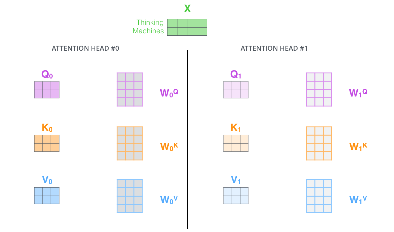
Multi-head attention. Each head has its own W_Q, W_K, W_V — the model gets several independent "views" of the sequence. Source: Jay Alammar — The Illustrated Transformer.

Around every attention block and every feed-forward block, you wrap a residual connection and layer normalisation — this is what makes the network trainable at depth. A modern LLM is basically N identical transformer blocks stacked on top of each other, with the same shape repeating: attention, residual + norm, feed-forward, residual + norm, next block.

Interview angle. Be ready to (a) write the attention formula from memory, (b) explain why we divide by $\sqrt{d_k}$ (to keep the softmax from saturating), and (c) explain the difference between self-attention and cross-attention. Self-attention is Q, K, V all coming from the same sequence. Cross-attention is Q from one sequence, K and V from another — this is how a decoder attends to an encoder in translation. Red flag to avoid: saying "attention weights are learned parameters." They're not — the weights come from softmax over the current input. The projection matrices $W_Q, W_K, W_V$ are learned; the attention scores are computed fresh for every input.

3. Tokens and context window

The transformer doesn't see characters or words. It sees tokens — chunks of characters, usually a subword. The word unhappiness might be one token, or it might be split into un + happi + ness, depending on how frequent the whole word was in training.

The tokenisation algorithm most modern LLMs use is Byte-Pair Encoding (BPE). Start with every character as a token. Then repeatedly merge the most frequent adjacent pair of tokens into a new token, until you hit a target vocabulary size (usually 30k–100k). Frequent words stay whole; rare words get broken into pieces; the vocabulary is fixed but you can still handle any input.

# What tokenisation actually looks like
import tiktoken

enc = tiktoken.get_encoding("cl100k_base")  # what GPT-4 uses
tokens = enc.encode("The interviewer asked about tokens.")
print(tokens)
# [791, 89568, 4691, 922, 11460, 13]

for t in tokens:
    print(t, repr(enc.decode([t])))
# 791    'The'
# 89568  ' interviewer'
# 4691   ' asked'
# 922    ' about'
# 11460  ' tokens'
# 13     '.'

Notice how " interviewer" includes the leading space. That's not a bug — BPE encodes spaces into the token, so "interviewer" at the start of a sentence and " interviewer" in the middle are technically different tokens.

Context window

The context window is the maximum number of tokens the model can process at once — prompt plus generation, combined. Everything the model "knows" for that call has to fit in there. GPT-3 shipped with 2048 tokens. GPT-4 Turbo has 128k. Claude 3.5 Sonnet has 200k. Some models now advertise 1M+. As a rough conversion, one English token is about 3/4 of a word, so 8k tokens ≈ 6000 words ≈ a short novella.

Attention is $O(n^2)$ in the sequence length because every token attends to every other token. That's why longer context was hard for a long time — a 128k-token forward pass would cost $128000^2 \approx 1.6 \times 10^{10}$ pairwise dot products per layer. Modern long-context models use tricks like FlashAttention, sparse attention, and sliding windows to keep this tractable.

Positional encoding

Attention itself is permutation-invariant — if you shuffle the input tokens, you get the same weighted sums out. That's a problem, because language cares about order. So you add a positional encoding to each token embedding before it goes into the first attention block. The original transformer used fixed sinusoidal encodings. Modern LLMs use RoPE (Rotary Position Embedding — rotates the Q and K vectors by an angle proportional to position, which extrapolates better to longer sequences) or ALiBi (Attention with Linear Biases — subtracts a linear penalty from attention scores based on token distance, no learned position embeddings at all). Both give the model a sense of "how far apart are these two tokens?" without hardcoding a maximum length.

Interview angle. If they ask about the context window, be able to say why it's expensive (quadratic attention), and mention RoPE or ALiBi if positional encoding comes up. If they ask "how many tokens is this sentence?" — reach for tiktoken, don't guess. A common trap: candidates confuse context window (max tokens per call) with training context length (how long the sequences were during pretraining). Models can sometimes be extended past their training context via RoPE scaling, but performance degrades past what they saw during training.

4. The three-stage post-training pipeline

This is the concept the interviewer wants you to nail because it's what turns a raw next-token predictor into something you'd actually want to talk to. A base LLM out of pretraining will happily continue a sentence, but it won't follow instructions, it won't refuse harmful requests, and it will happily produce whatever comes next in its training distribution — which might not be what you asked for.

The pipeline that fixes this has three stages: pretraining → supervised fine-tuning (SFT) → reinforcement learning from human feedback (RLHF), or its increasingly popular replacement, DPO.

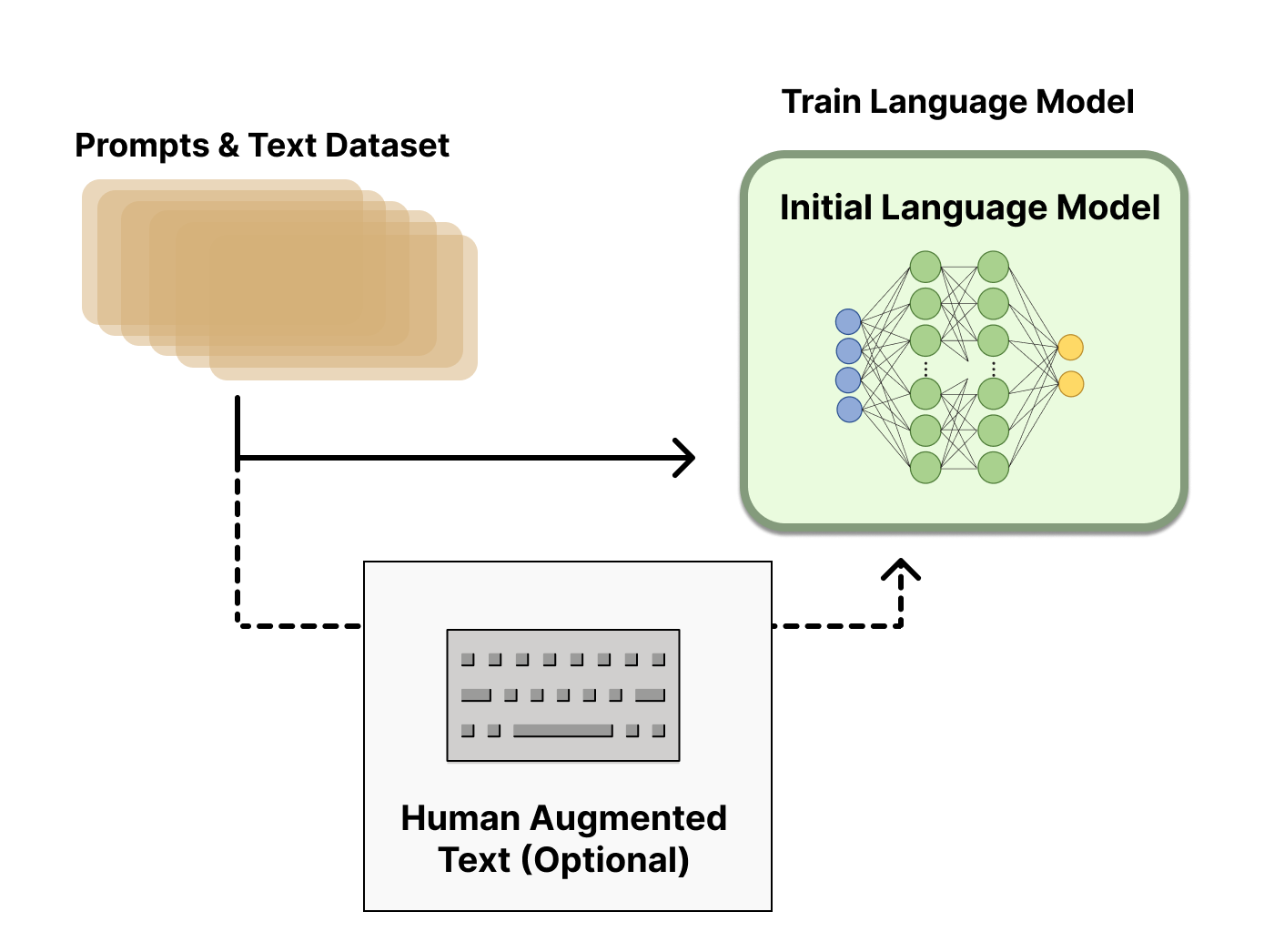
Stage 1: pretraining. Diagram from Hugging Face — Illustrating RLHF.

Stage 1 — Pretraining

Self-supervised next-token prediction on a huge corpus of internet text, books, code, and whatever else you can scrape. Objective: minimise cross-entropy on next-token prediction. Output: a base model that has absorbed language, facts, code, and reasoning patterns — but doesn't yet know how to be an assistant. If you prompt a base model with "What is the capital of France?", it might reply with "What is the capital of Germany? What is the capital of Italy?" — because the most likely next tokens after that question are more questions in a quiz-style continuation.

Stage 2 — Supervised Fine-Tuning (SFT)

Take a smallish dataset of high-quality (prompt, response) pairs written by humans. Fine-tune the base model on these using the same next-token objective, but now the completions look like helpful answers instead of internet noise. Output: a model that follows instructions and produces answer-shaped responses. This is also called instruction tuning.

Stage 3a — Reward model + PPO (classic RLHF)

SFT gets you a lot of the way, but you can go further by teaching the model preference. This is where RLHF comes in. It has two sub-stages:

Train a reward model. For each prompt, ask humans to rank several model responses from best to worst. Train a separate neural network (usually a copy of the LLM with a scalar head on top) to predict which of two responses a human would prefer. The reward model outputs a single scalar — higher means "humans like this response more."

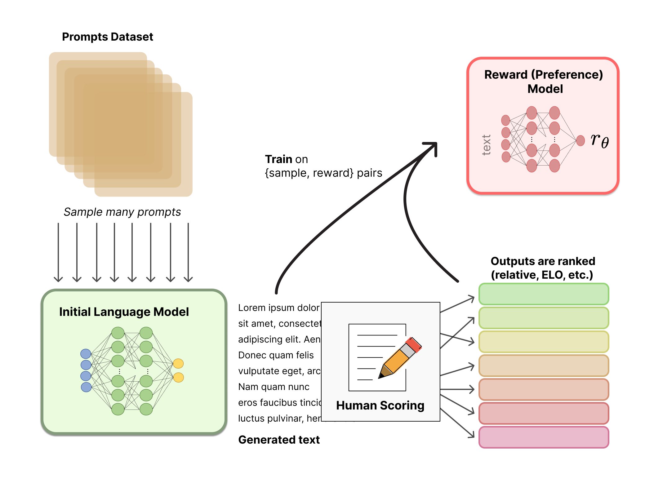
Training a reward model from human preference rankings

Reward model training. Humans rank pairs of responses; the reward model learns to score any response the way humans would. Source: Hugging Face — Illustrating RLHF.

Fine-tune with PPO. Now use the reward model as a reward signal in a reinforcement learning loop. Proximal Policy Optimization (PPO) updates the LLM to produce responses the reward model scores highly, while adding a KL penalty against the SFT model to stop the policy from drifting too far from sensible language. Without the KL term, the model gaming the reward model produces gibberish that scores well but is unreadable (this is called reward hacking).

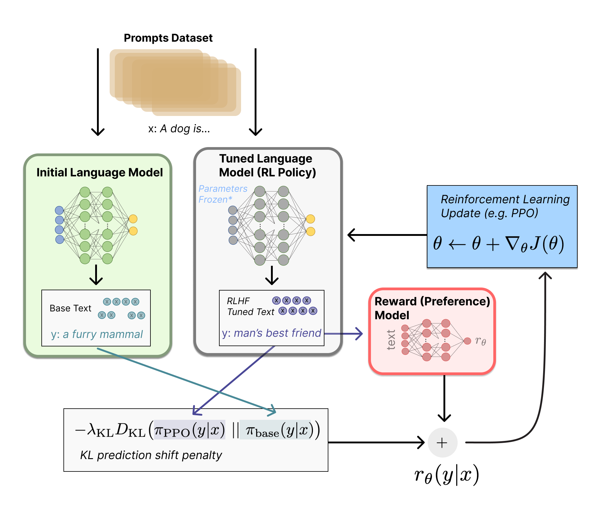
Full three-stage RLHF pipeline: pretraining, supervised fine-tuning, reward model, PPO

The full RLHF loop. The SFT model is copied twice — once frozen (reference for the KL penalty), once trained by PPO against the reward model. Source: Hugging Face — Illustrating RLHF.

This is the recipe made famous by OpenAI's InstructGPT paper, which was the direct ancestor of ChatGPT.

Stage 3b — DPO (the alternative)

RLHF works, but it's a nightmare to implement. Two extra models in memory (the reward model and the frozen reference), an unstable RL loop, hyperparameter sensitivity. In late 2023, Rafailov et al. proposed Direct Preference Optimization (DPO), which skips the reward model entirely.

The insight: instead of training a reward model to predict human preferences and then doing RL against it, you can derive a closed-form loss that directly optimises the policy on the preference pairs. The math shows that the optimal policy under RLHF has a specific relationship to the reference policy and the reward — you can rearrange that relationship into a supervised loss that only needs (prompt, chosen, rejected) triples.

\mathcal{L}_{\text{DPO}} = -\mathbb{E}\left[\log \sigma\left(\beta \log \frac{\pi_\theta(y_w|x)}{\pi_{\text{ref}}(y_w|x)} - \beta \log \frac{\pi_\theta(y_l|x)}{\pi_{\text{ref}}(y_l|x)}\right)\right]

Where $y_w$ is the winner, $y_l$ the loser, $\pi_\theta$ the current policy, $\pi_{\text{ref}}$ the SFT model, and $\beta$ a hyperparameter controlling how far you can drift. It looks scary but it's just binary cross-entropy on preference pairs.

RLHF vs DPO at a glance:

Property	RLHF (PPO)	DPO
Extra model needed	Reward model	None
Loop type	RL (unstable)	Supervised (stable)
Compute	High	Low
Preference data format	Rankings or pairs	Pairs only
Implementation complexity	High	Low
Where it shines	Very large scale, careful tuning	Practical alignment for most teams

Interview angle. Almost guaranteed question. Be able to walk through all three stages (pretrain → SFT → RLHF or DPO), what data each stage needs (raw text → instruction pairs → preference pairs), and why the KL penalty exists in PPO. If they ask about DPO, mention that it replaces the reward-model + PPO stack with a single supervised loss, and that this is why most open-source alignment work in 2024–2025 uses DPO or one of its variants (IPO, KTO, ORPO).

5. Sampling and decoding

Once the model is trained, you still have to decide how to use it. Every forward pass gives you a probability distribution over the next token. Sampling is the algorithm that picks one.

Greedy decoding

Take the token with the highest probability every time. Deterministic. Often produces bland, repetitive output — because the highest-probability continuation is usually a common phrase, which loops back on itself.

Temperature

Divide the logits by a temperature $T$ before softmax:

p_i = \frac{\exp(z_i / T)}{\sum_j \exp(z_j / T)}

$T = 1$ : default distribution.
$T \to 0$ : distribution collapses onto the argmax (equivalent to greedy).
$T > 1$ : distribution flattens, low-probability tokens get more chance.

Temperature = 0 for factual QA (you want the most likely answer). Temperature = 0.7–1.0 for creative writing. Temperature = 1.5+ almost always turns into word salad.

Top-k sampling

Only sample from the top $k$ most likely tokens. Everything else gets zeroed out. $k = 50$ is a common default. Keeps the model from picking something absurd from the long tail.

Top-p (nucleus) sampling

Introduced in Holtzman et al. 2019. Instead of a fixed $k$ , take the smallest set of tokens whose cumulative probability exceeds $p$ . If $p = 0.9$ , you sample from whatever tokens make up the top 90% of probability mass. The nucleus adapts — when the model is confident, only a few tokens are in the pool; when uncertain, more.

Top-k vs top-p sampling comparison showing how each restricts the token pool

How top-k and top-p carve up the probability distribution differently. Source: Sebastian Raschka — Temperature, top-k, top-p FAQ.

Almost every modern deployment applies temperature first, then top-p on the reshaped distribution. Sometimes both top-k and top-p are used as guardrails.

# What this looks like in the OpenAI API
from openai import OpenAI
client = OpenAI()

response = client.chat.completions.create(
    model="gpt-4o",
    messages=[{"role": "user", "content": "Write one line about the sea."}],
    temperature=0.8,   # creativity dial
    top_p=0.9,         # nucleus
    max_tokens=50,
)

Sampling comparison, at a glance:

Strategy	What it does	Good for	Downside
Greedy ( $T=0$ )	Argmax every step	Factual QA, code	Repetitive, bland
Temperature	Rescales logits before softmax	Creativity dial	Alone, can produce gibberish
Top-k	Keep top $k$ tokens	Trims long tail	Rigid — same $k$ regardless of confidence
Top-p (nucleus)	Keep smallest set > $p$ mass	Adaptive, most common in prod	Extra hyperparam

Interview angle. If they ask "how do you make the model less random?", say temperature toward 0, or top-p toward a small value like 0.1. If they ask "what does temperature = 0 mean?", say it's equivalent to greedy decoding — deterministic argmax. Red flag: don't confuse temperature (softmax scaling) with top-p (probability mass truncation) — they're orthogonal knobs and you often use both.

6. Prompt structure: system, user, assistant

Modern chat LLMs don't take raw text. They take a chat template — a structured sequence of messages, each with a role. Three roles matter:

system — the frame. Persona, task, constraints, output format. Sent once at the start. This is where you write "You are a helpful assistant. Reply only in JSON." The system prompt has the strongest influence on model behaviour.
user — what the user typed. The actual question or task.
assistant — what the model said (or should say). In multi-turn conversations, previous assistant messages get replayed here as context.

messages = [
    {"role": "system", "content": "You are a terse Python tutor. Reply in <=3 lines."},
    {"role": "user",   "content": "How do I read a CSV in pandas?"},
    {"role": "assistant", "content": "import pandas as pd\ndf = pd.read_csv('file.csv')"},
    {"role": "user",   "content": "How do I show the first 5 rows?"},
]

response = client.chat.completions.create(model="gpt-4o", messages=messages)

Notice the assistant message in the middle — that's how you give the model a memory of what it said before, so the next answer stays consistent with the "terse tutor" persona.

Interview angle. If they ask about prompt structure, mention the three roles and what each is for. If they ask about prompt injection (which will come up in Part 8 of this series), the system prompt is where the vulnerability lives — a user message that says "ignore the above instructions" can sometimes override the system message. That's why role separation is a security concern, not just a formatting concern.

7. In-context learning: zero-shot, one-shot, few-shot

One of the most surprising things about LLMs is that they can learn a task at inference time, just by showing examples in the prompt. No gradient updates. No fine-tuning. This is called in-context learning, and it's the phenomenon that made GPT-3 famous.

Zero-shot. No examples. Just the instruction. "Translate to French: I love bread."
One-shot. One example, then the query. "English: Hello → French: Bonjour. English: I love bread → French: "
Few-shot. Two to a few dozen examples. Same idea, more demonstrations.

The GPT-3 paper was subtitled "Language Models are Few-Shot Learners" precisely because they showed that as models scale up, few-shot performance improves dramatically — sometimes even matching fine-tuned models. This was the moment the field pivoted from "fine-tune a smaller model for every task" to "prompt one big model for every task."

The mechanism isn't fully understood. It looks like the model is doing implicit gradient descent inside its forward pass on the examples you provide — but it's more like pattern completion than actual learning. Either way, empirically it works.

# Few-shot classification without any fine-tuning
prompt = """Classify the sentiment as positive, negative, or neutral.

Text: This movie was a waste of two hours.
Sentiment: negative

Text: Perfectly fine, nothing memorable.
Sentiment: neutral

Text: I could not stop smiling the whole time.
Sentiment: positive

Text: The plot was confusing but the acting was excellent.
Sentiment:"""

Interview angle. If they ask "how do you get the model to do a new task without fine-tuning?", the answer is few-shot prompting. Mention that GPT-3 showed few-shot performance improves with scale, and that in-context learning is a big reason why LLMs are used as generalists rather than specialists. Red flag: don't call this "training" — no weights change during in-context learning. It's conditioning, not learning in the gradient-descent sense.

8. Chain-of-thought prompting (basics)

Reasoning-heavy questions — arithmetic, logic puzzles, multi-hop questions — are where LLMs used to fall apart. Wei et al. 2022 found something almost embarrassingly simple: if you show the model examples where the answer includes the intermediate reasoning steps, and then ask a new question, the model starts producing intermediate reasoning steps too — and its accuracy jumps.

The classic example from the paper:

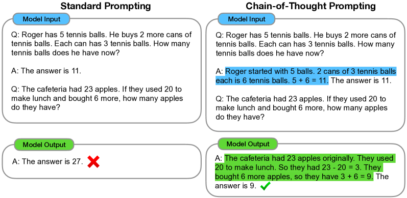
Chain-of-thought prompting example from Wei et al. 2022 showing standard prompting vs chain-of-thought prompting

Left: standard prompting gives the answer directly and gets it wrong. Right: chain-of-thought prompting shows the reasoning first, and gets it right. Source: Wei et al. 2022 — Chain-of-Thought Prompting Elicits Reasoning in Large Language Models.

The variant Kojima et al. 2022 showed also works: zero-shot CoT. Just append "Let's think step by step." to any question, and a sufficiently large model will produce a reasoning trace and often get the right answer.

# Zero-shot CoT
prompt = """Q: Roger has 5 tennis balls. He buys 2 more cans of tennis balls.
Each can has 3 balls. How many tennis balls does he have now?
A: Let's think step by step."""

Chain-of-thought is only the tip of the iceberg — self-consistency, tree-of-thoughts, ReAct, planner-executor patterns are all built on this idea of making the model write down its reasoning. Part 6 of this series goes deep on the whole family.

Interview angle. Be ready to explain why CoT works (it lets the model use its later tokens to condition on earlier reasoning — the extra compute is what buys the accuracy), and when it doesn't (small models, tasks that don't decompose into steps, cases where the model hallucinates confident-but-wrong reasoning). Also mention: CoT trades tokens for accuracy. If your budget is tight, it costs you.

9. Scaling laws and emergent behaviour

The last big idea. Why did all of this suddenly work around 2020? Because we discovered that LLM performance scales predictably with three things: parameters ( $N$ ), data ( $D$ ), and compute ( $C$ ).

Kaplan et al. 2020 — OpenAI. Loss follows a power law: $L(N, D, C) \propto \text{stuff}^{-\text{small exponent}}$ . Bigger is better, and you can predict the loss of your next training run before you do it.
Hoffmann et al. 2022 — DeepMind (Chinchilla). The refinement. Kaplan overestimated the value of parameters and underestimated the value of data. For a fixed compute budget, the compute-optimal recipe is to scale parameters and tokens roughly equally — about 20 tokens per parameter is the sweet spot. Chinchilla was a 70B model trained on 1.4T tokens; it beat Gopher (280B on 300B tokens), a model 4x its size, because Gopher was under-trained.
Wei et al. 2022 on emergent abilities. Some capabilities don't scale smoothly — they jump. At a certain parameter count, few-shot arithmetic goes from near-zero to solid overnight. Same for word unscrambling, some kinds of reasoning, following complex instructions. There's ongoing debate about whether these are true phase transitions or artefacts of how the metrics are measured, but empirically the effect is real.

Interview angle. If they mention Chinchilla, the punchline is most pre-2022 LLMs were over-parameterised and under-trained; the fix was more data, not more parameters. If they ask about emergent abilities, be able to name a few (arithmetic, in-context learning quality, following multi-step instructions) and mention that this is why bigger models aren't just quantitatively better — they can be qualitatively better. Trap to avoid: don't say "the model becomes conscious" or anything mystical. Emergent means "not present at small scale, present at large scale." That's it.

Common interview questions (with model answers)

Q1: What's the difference between an encoder-only, decoder-only, and encoder-decoder transformer? Encoder-only (BERT) processes the whole sequence bidirectionally — every token attends to every other token, no masking. Best for classification, embedding, retrieval. Decoder-only (GPT) uses causal masking — every token only attends to previous tokens. Best for generation. Encoder-decoder (T5, original transformer) has both: the encoder processes the input bidirectionally, the decoder generates output while cross-attending to the encoder output. Best for translation and seq2seq tasks. Modern chat LLMs are almost all decoder-only.

Q2: Why do we divide by root d_k in attention? Without it, the dot products $Q K^T$ scale with $d_k$ (variance grows linearly). Large scores push the softmax into a saturated regime where one weight is ≈1 and the rest are ≈0, which kills gradients. Dividing by $\sqrt{d_k}$ keeps the variance of the scores constant regardless of head dimension.

Q3: Explain the three-stage post-training pipeline. Stage 1 is pretraining on raw internet text with a next-token objective — this gives you a base model that knows language but isn't an assistant. Stage 2 is supervised fine-tuning on curated (prompt, response) pairs written by humans — this teaches it to follow instructions. Stage 3 is preference tuning, either RLHF (train a reward model on human rankings, then use PPO with a KL penalty against the SFT model) or DPO (skip the reward model, directly optimise the policy on preference pairs with a supervised loss). Stage 3 is what makes the model helpful and harmless, not just fluent.

Q4: What's the difference between top-k and top-p sampling? Top-k keeps a fixed number of the most likely tokens regardless of the shape of the distribution — always exactly $k$ . Top-p (nucleus) keeps the smallest set of tokens whose cumulative probability exceeds $p$ — so the number of tokens adapts. When the model is confident, top-p is narrow; when uncertain, it widens. Top-p is generally preferred for open-ended generation because it's adaptive; top-k is a simpler fallback.

Q5: Why is DPO replacing RLHF? RLHF requires training a separate reward model and running an unstable RL loop with PPO, plus keeping a frozen reference model in memory for the KL penalty. DPO derives a closed-form loss that lets you optimise the same objective with plain supervised learning on preference pairs — no reward model, no RL, no reference model at inference (only at training). It's simpler, more stable, and empirically matches or beats RLHF at practical scales. Most open-source alignment in 2024–2025 uses DPO or one of its variants (IPO, KTO, ORPO).

Q6: What happens if I set temperature = 0? It collapses the softmax distribution onto the argmax token. In practice this is equivalent to greedy decoding — deterministic, most-likely-token every step. You use this for factual QA, code generation, or anywhere you want reproducibility. But it tends to produce repetitive text and can get stuck in loops for open-ended generation.

Q7: What is a KL penalty in RLHF and why does it exist? The reward model isn't perfect — the policy can find high-reward outputs that are actually nonsense (reward hacking). The KL divergence between the current policy and the SFT reference policy is added to the objective as a penalty, keeping the policy from drifting too far from something that produces reasonable language. It's the "don't get too weird" term. In DPO, the equivalent role is played by the $\beta$ hyperparameter and the reference-policy log-ratio in the loss.

What to read next

The natural next post is Part 6: Prompting and reasoning loops — chain-of-thought in depth, self-consistency, tree-of-thoughts, ReAct, and the planner-executor pattern. Everything the interviewer will ask once they're satisfied you understand the model. That builds directly on the CoT basics from section 8 above.

If any of the language modelling foundations felt fuzzy — n-grams, perplexity, RNNs, BERT vs GPT, transfer learning — the deeper walkthrough is in NLP Part 5: Language Modeling. It covers the arc from document-term matrices through Word2Vec, RNNs, ELMo, transformers, BERT, and GPT-3, and it's the post to read alongside this one if you want the "how did we get here" story.

The four-page revision sheet that summarises everything above (and everything coming later in the series) lives at the GenAI Interview Prep Cheatsheet. Read this post to understand it; print that one for the train.