Cheat sheet

Part 5 · Language Modeling — Cheat Sheet

Four illustrated pages — the representation arc, probability and n-grams, neural language models, transformers and GPT-3.

Part 5 · Language Modeling — Cheat Sheet — printable cheat sheet
Download PNG

Or read the searchable version below.

Page 1 · Opening + Word2Vec → Language Models
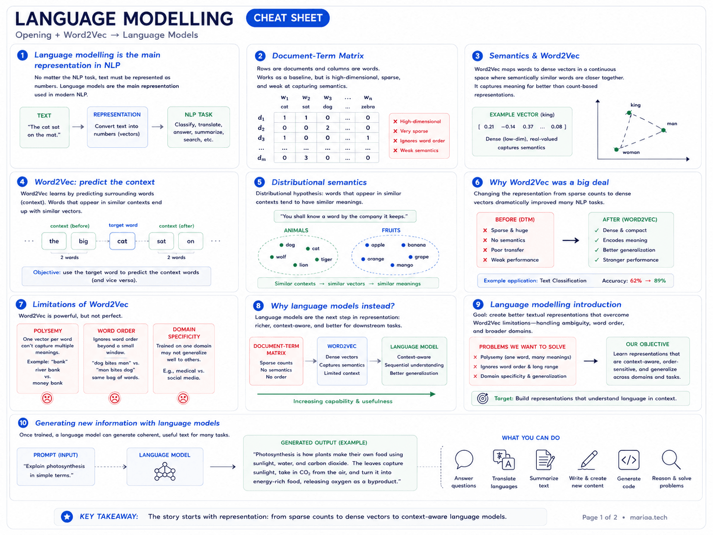
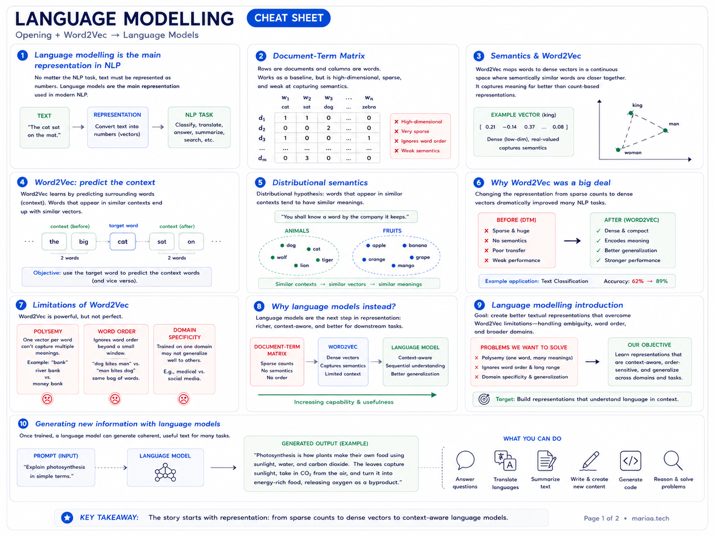
Page 1 of 4 of the language-modeling cheatsheet. Ten cards covering the representation arc that leads into language modeling: (1) language modeling is the main representation in NLP — every task needs to turn text into numbers, classify/translate/answer/summarise on top; (2) document-term matrix baseline — rows are documents, columns are words, sparse and weak at semantics; (3) semantics with Word2Vec — dense vectors place semantically similar words close together (king/man/woman example); (4) Word2Vec predicts the context — target word predicts surrounding words; (5) distributional semantics — 'you shall know a word by the company it keeps', animals vs fruits clusters; (6) why Word2Vec was a big deal — sparse counts to dense vectors, better generalisation, text classification jumps from 62% to 89%; (7) limitations of Word2Vec — polysemy (bank), word order ('dog bites man' vs 'man bites dog'), domain specificity; (8) why language models instead — DTM → Word2Vec → language model, increasing capability and usefulness; (9) language modeling introduction — goal is context-aware, order-sensitive, generalising representations; (10) generating new information with language models — prompt in, coherent generated text out, answer/translate/summarise/code/reason.
The representation arc: from DTM to Word2Vec to language models. Each step solves a limitation the previous one couldn't.

Page 2 · Probability, n-grams, evaluation
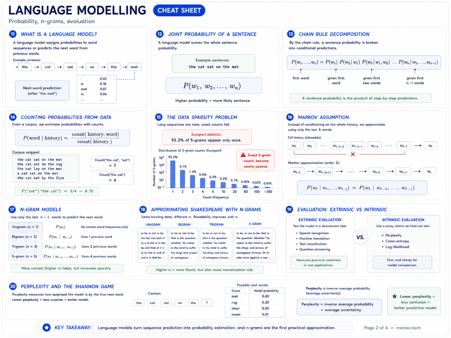
Page 2 of 4. Ten cards: (11) what is a language model — assigns probabilities to word sequences or predicts the next word; (12) joint probability of a sentence — P(w_1, w_2, ..., w_n); (13) chain rule decomposition — P(w_1..w_n) = P(w_1) P(w_2|w_1) ... P(w_n|w_1..w_{n-1}); (14) counting probabilities from data — P(word | history) ≈ count(history, word) / count(history); (15) the data sparsity problem — Europarl statistic, 92.2% of 5-grams appear only once; (16) Markov assumption — approximate using only the last k words, P(w_t | w_1..w_{t-1}) ≈ P(w_t | w_{t-k}..w_{t-1}); (17) n-gram models — unigram/bigram/trigram/5-gram, more context helps but increases sparsity; (18) approximating Shakespeare with n-grams — same training data at n=1..5, higher n is more fluent but memorises; (19) evaluation extrinsic vs intrinsic — downstream task vs perplexity/cross-entropy/log-likelihood; (20) perplexity and the Shannon game — lower perplexity = less surprise = better model.
From joint probability to perplexity. Chain rule, Markov assumption, n-grams, and the two evaluation modes — extrinsic on a downstream task vs intrinsic via perplexity.

Page 3 · Neural language models, contextual embeddings, attention
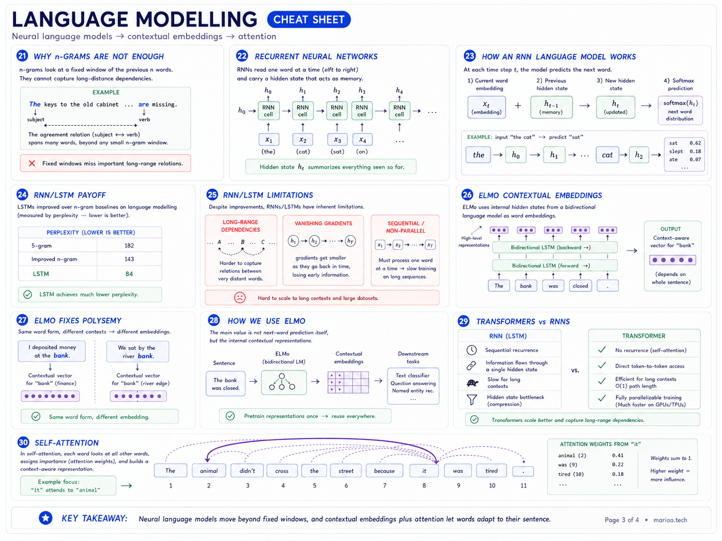
Page 3 of 4. Ten cards: (21) why n-grams are not enough — fixed window misses long-range subject-verb agreement ('The keys to the old cabinet ... are missing'); (22) recurrent neural networks — read one word at a time, carry a hidden state, RNN cells chained left to right; (23) how an RNN language model works — at each step t use current embedding x_t plus previous hidden state h_{t-1} to produce h_t and softmax over the next word; (24) RNN/LSTM payoff — perplexity drops from 5-gram 182 to improved n-gram 143 to LSTM 84; (25) RNN/LSTM limitations — still struggle with long-range dependencies, vanishing gradients, sequential and non-parallelisable; (26) ELMo contextual embeddings — internal hidden states from a bidirectional LSTM used as word embeddings; (27) ELMo fixes polysemy — 'I deposited money at the bank' vs 'We sat by the river bank' yield different contextual vectors; (28) how we use ELMo — feed the bidirectional LM's internal representations into downstream classifiers, pretrain once and reuse; (29) transformers vs RNNs — no recurrence, direct token-to-token access, parallelisable, O(1) path length; (30) self-attention — every word looks at every other word ('it' attends to 'animal'), attention weights sum to 1.
The neural era. RNNs and LSTMs cracked sequential modeling, ELMo turned hidden states into context-aware embeddings, and self-attention removed recurrence entirely.

Page 4 · BERT, transfer learning, GPT-3, distillation

Page 4 of 4. Eleven cards: (31) why transformers are a big deal — no recurrence, direct long-range connections, parallel processing, multiple attention heads; (32) BERT masked language modeling — predict masked tokens from context ('The cat sat on the [MASK]' → mat 0.72); (33) BERT is bidirectional — uses both left and right context simultaneously, unlike causal left-to-right; (34) BERT creates strong representations — pretrained BERT fine-tuned for classification, NER, QA, sentence-pair tasks; (35) training cost of large language models — thousands of GPUs, BERT around $250k in 2018, significant carbon footprint; (36) transfer learning in NLP — stage 1 pretrain on huge raw text, stage 2 fine-tune on smaller labeled dataset; (37) why transfer learning matters — model doesn't relearn syntax/semantics/discourse/world knowledge from scratch every task; (38) GPT-3 and zero-shot learning — large models perform tasks directly from prompts, no gradient updates; (39) prompting as task framing — translation, sentiment, summarisation, QA all framed as next-word prediction with the right prompt; (40) model distillation — smaller student mimics larger teacher, keep most of the performance with far fewer parameters; (41) the full arc of language modeling — probability over sequences → n-grams → RNN/LSTM → ELMo → Transformer → BERT → GPT-3 → distillation.
From attention to scale. Pretraining and fine-tuning replaced training-from-scratch; GPT-3 replaced fine-tuning with prompts; distillation made it deployable.