When Missing Values Aren't Random

Last update: February 2024. All opinions are my own.

A binary classification competition from Kaggle: predict whether a passenger aboard the Spaceship Titanic was transported to another dimension after the ship collided with a spacetime anomaly. Submissions are graded on classification accuracy.

The interesting part of this dataset isn't the model. It's the schema: PassengerIDs encode travel groups, Cabins encode physical location on the ship, and large chunks of the data are missing. The trick is realising that most of the missing values can be recovered by reading the structure of the data itself — not by filling with means.

1. The fields you start with

2. What the missing values look like

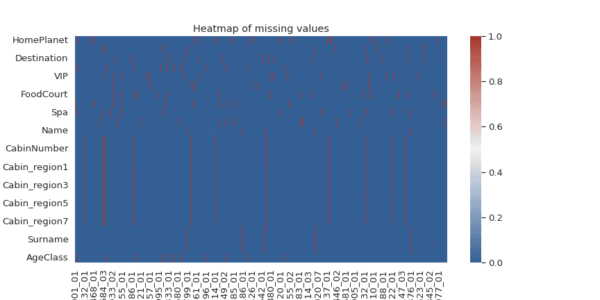
Almost every column has some missing data, but the missingness isn't random — it clusters around groups and cabins. That's important, because it means the right imputation strategy is relational, not statistical.

3. Decoding the schema before modelling

Three of the fields are composite — they're really multiple features glued together. Splitting them is the single biggest source of signal.

3.1 PassengerID → group + position

df['PassengerGroup']   = df.index.str.split('_').str[0]
df['PassengerNumber']  = df.index.str.split('_').str[1].astype(int)
df['GroupSize']        = df.groupby('PassengerGroup')['PassengerGroup'].transform('count')
df['Solo']             = (df['GroupSize'] == 1).astype(int)

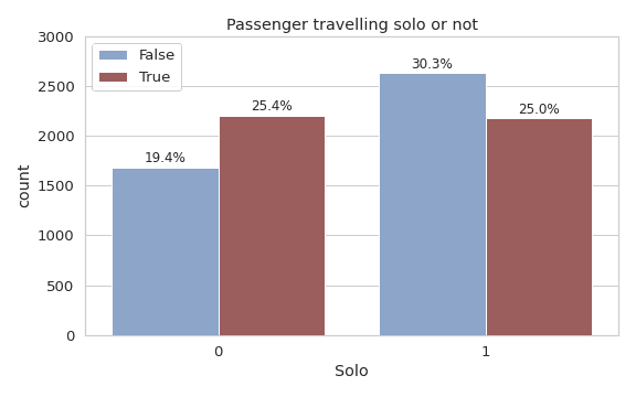
From PassengerId alone you can derive: the group, the size of the group, and whether the passenger is travelling alone. Solo ends up being a useful signal — solo travellers behave differently from family groups.

3.2 Cabin → deck + number + side

df[['CabinDeck', 'CabinNumber', 'CabinSide']] = df['Cabin'].str.split('/', expand=True)
df['CabinNumber'] = pd.to_numeric(df['CabinNumber'])
df['cabin_region'] = pd.cut(df['CabinNumber'], bins=6, labels=range(6))

Cabin looks like B/12/P — a deck letter, a number along the deck, and a side. Each piece carries its own signal: deck correlates with HomePlanet, side correlates with travel group, and cabin_region (the cabin number binned) helps because adjacent passengers tend to share characteristics.

3.3 Name → surname → family

df['Surname'] = df['Name'].str.split(' ').str[-1]
df['FamilySize'] = df.groupby('Surname')['Surname'].transform('count')

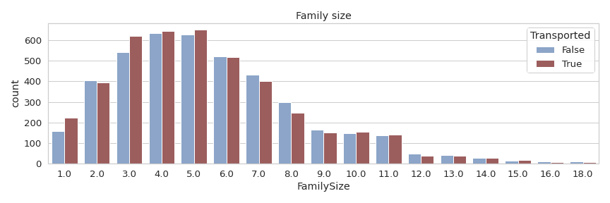
Same idea as Group, but using surname. Where multiple groups share a surname, you have a family travelling together — useful both as a feature and for imputing missing values inside the family.

3.4 Expenditure → total, none, luxury, basic

The five amenity-spending columns roll up nicely:

• TotalExpenditure = sum of all spending.
• NoExpenditure = boolean: did they spend anything at all?
• LuxuryExpenditure = RoomService + Spa + VRDeck.
• BasicExpenditure = FoodCourt + ShoppingMall.

NoExpenditure is the most important of these — and it's the bridge to imputing CryoSleep, which we'll see in a moment.

4. Imputing missing values by reading the data

This is where the project gets interesting. Instead of filling missing values with means or modes, I imputed using inter-feature relationships that the schema implies. Almost every relationship is something a human would notice if they looked at the data carefully.

4.1 HomePlanet — fill from travel companions

Travel groups almost always share a HomePlanet. If anyone in a group has a known HomePlanet, propagate it to the rows in that group with missing HomePlanet. Same with families (surname).

df['HomePlanet'] = df.groupby('PassengerGroup')['HomePlanet'].transform(
    lambda x: x.fillna(x.mode().iloc[0]) if not x.mode().empty else x
)

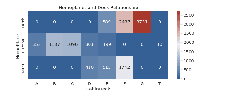
Then fall back to the CabinDeck → HomePlanet relationship. Most decks are dominated by one HomePlanet:

4.2 Cabin — fill from group and surname

CabinSide (P/S) is almost perfectly preserved within travel groups — if any group member has a known side, the others share it. Same for surname.

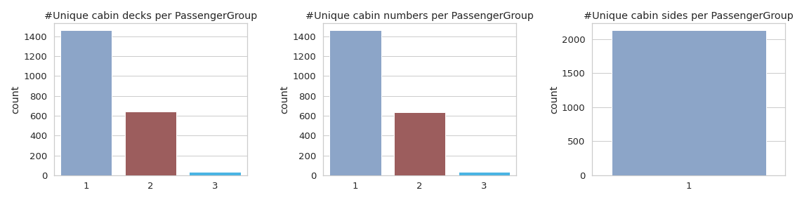
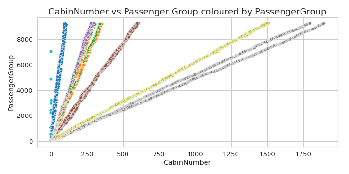
For missing CabinNumber, the cabin numbers within a deck are mostly contiguous. So I fitted a small linear regression on cabin number vs passenger index (per deck) to fill the rest:

4.3 CryoSleep — derive from spending

The dataset description says CryoSleep passengers are confined to their cabins. They cannot spend anything. So:

Conversely, if CryoSleep == True and any spending column is missing, the missing values should be filled with 0, not the column mean. This single rule cleans up a chunk of the dataset.

4.4 VIP, Age, Surname, Destination

Each of these gets a similar relational treatment:

• VIP → mostly correlated with HomePlanet (one planet has disproportionately more VIPs), then refined by age class.
• Age → median age within group, then within deck.
• Surname → fill within group (same group → same family → same surname).
• Destination → mode within group, then by HomePlanet.

5. What the data looks like once cleaned

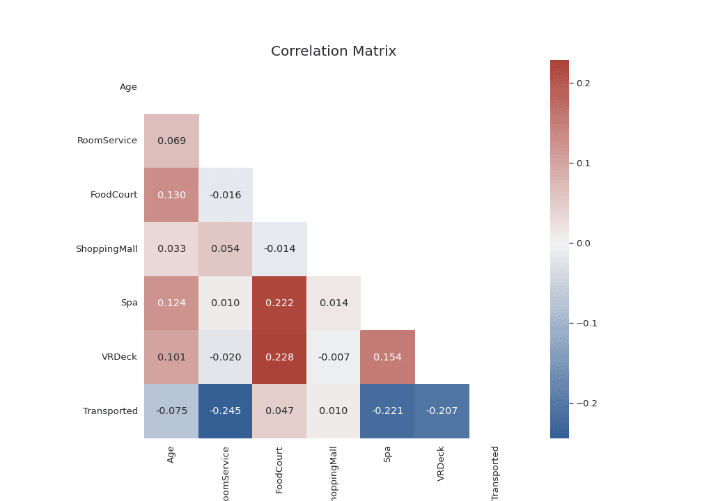
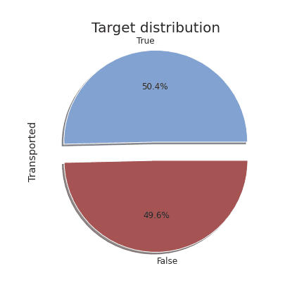
Before modelling, a quick sanity check on correlations:

6. Modelling — 10 classifiers, one preprocessing pipeline

With the data cleaned and engineered, the modelling part was almost mechanical: build a single preprocessing pipeline, plug it into a column transformer, then fit ten classifiers on the same train/validation split and compare cross-validation scores.

classifiers = {
    'Naive Bayes':         GaussianNB(),
    'Logistic Regression': LogisticRegression(C=0.2, solver='liblinear'),
    'SGD Classifier':      SGDClassifier(loss='log'),
    'Decision Tree':       DecisionTreeClassifier(max_depth=7),
    'SVC':                 SVC(random_state=0, probability=True),
    'Random Forest':       RandomForestClassifier(max_depth=7, n_estimators=100),
    'AdaBoost':            AdaBoostClassifier(n_estimators=100),
    'CatBoost':            CatBoostClassifier(iterations=10, learning_rate=0.1, verbose=False),
    'LightGBM':            lgb.LGBMClassifier(learning_rate=0.05, n_estimators=500, reg_lambda=1),
    'XGBoost':             XGBClassifier(),
}

The preprocessing pipeline was identical for every model — standardise the continuous columns, one-hot encode the categorical ones, leave the booleans alone:

preprocessor = ColumnTransformer(transformers=[
    ('num', Pipeline([('scaler', StandardScaler())]),
            make_column_selector(dtype_include=np.number)),
    ('cat', Pipeline([('onehot', OneHotEncoder(handle_unknown='ignore', sparse=False))]),
            make_column_selector(dtype_include=['category', 'object'])),
])

After cross-validation:

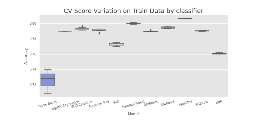
The boosted models (LightGBM, XGBoost, CatBoost) and Random Forest sit at the top. Linear models perform respectably but are clearly outclassed once the dataset has 30+ engineered features.

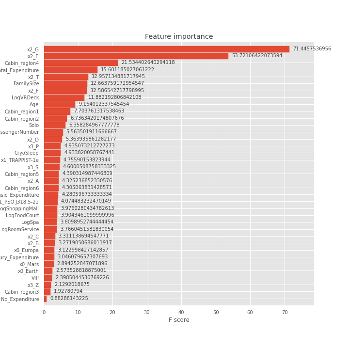
The top features are almost all engineered. CryoSleep, TotalExpenditure / NoExpenditure, and the Cabin splits do most of the work. The raw columns barely appear in the top of the chart — which validates the upfront investment in unpacking the schema.

7. What I'd take into the next dataset

A few other things I'd repeat:

• Read the field descriptions. "CryoSleep passengers are confined to their cabins" is a single sentence that gives you a free imputation rule for hundreds of rows.
• Don't fill missing values with statistics if you can fill them with relationships. Group, family, deck, and side are all schema-level hints that beat a column-wise mean fill.
• Build one preprocessing pipeline, then race models. Once the data is clean, a 10-model bake-off is almost free. The model that wins is rarely the one you'd have picked first.

Related Kaggle write-ups

Two other walkthroughs in the same series — every one starts with feature semantics before any model:

• Before You Fix Your Data, Understand It (Forest Cover Type) — cartographic features, sanity checks, and why "weird values" often mean geography rather than bad data.
• Bike-Sharing Demand Forecasting — hourly demand in Washington, D.C., with cyclic time encodings and time-aware cross-validation.

Resources