Finding the Right Influencer with a Graph

Last update: December 2023. All opinions are my own.

A team project (Group A, IE MBD, December 2023) for a fictional shoe brand called Botas. The brief: identify the Instagram account that would produce the most sales if Botas sponsored a single post. The interesting part isn't the marketing argument — it's the network analysis underneath: how to shrink a 70k-node graph without flattening it, which centrality measure actually answers the question, and what diffusion modelling adds on top of static metrics.

1. The brief and the data

Botas wanted one influencer. The temptation is to pick whoever has the most followers and stop there — but follower count is a property of a single node. Influence is a property of a node's position in a network, and the only way to see position is to build the network.

The dataset was a Kaggle scrape of Instagram users, collected via the hashtags #iloveshoes, #niceshoes, and #shoes. Each row was an account with the kind of profile and engagement stats Instagram exposes:

70,409 vertices in total. With the edges between them, the raw graph was too large to run iterative centrality or community detection on in a reasonable time on Colab — so the first real decision was how to make it smaller.

2. Shrinking the graph without flattening it

So the reduction had to be structured, not random. The approach: cluster accounts on the profile-stats features (followers, engagement, growth, posting cadence), then keep accounts from the clusters that actually behave like community members rather than passive scrollers. This preserves the parts of the network that carry real follow-edges and discards the long tail of inactive accounts that contribute almost no structure.

A quick sanity check after reduction:

• Degree distribution kept its heavy tail — not flattened by the sampling.
• Average clustering coefficient stayed well above what a random graph of the same size would have.
• A handful of high-degree hubs were preserved (these end up mattering for both centrality and community detection).

3. Building the graph

The graph is a directed network — A follows B is not the same as B follows A — and the edges carry no weight. Two libraries, used in parallel: networkx (more readable code, easier ad-hoc plotting) and igraph (much faster on community detection and large-graph metrics).

import networkx as nx
import igraph as ig
import pandas as pd

vertices_df = pd.read_csv('data/Instagram User Stats_final.csv')
edges_df    = pd.read_csv('data/edges.csv')

G_nx = nx.from_pandas_edgelist(
    edges_df,
    source='source',
    target='target',
    create_using=nx.DiGraph,
)

G_ig = ig.Graph.TupleList(
    edges_df.itertuples(index=False),
    directed=True,
)

Same graph, two representations. Centrality and visualisation in networkx, community detection and global metrics in igraph.

4. The shape of the network

Before any algorithm, a handful of global metrics describe what kind of network we're looking at:

• Density — what fraction of possible edges actually exist. Social graphs are sparse; ours was no exception.
• Diameter — the longest shortest path between any two reachable nodes. A measure of how far news has to travel in the worst case.
• Average path length — the typical distance between two nodes. The famous "small-world" property: in real social networks, this is shockingly small.
• Transitivity (global clustering coefficient) — the probability that two friends of a node are also friends with each other. High transitivity = lots of triangles = community structure.
• Reciprocity — in a directed graph, the share of edges that are mutual (A follows B and B follows A). High reciprocity in a follow network suggests friendship rather than fan-base behaviour.

# global metrics on the reduced graph
metrics = {
    'density':       G_ig.density(),
    'diameter':      G_ig.diameter(),
    'avg_path_len':  G_ig.average_path_length(),
    'transitivity':  G_ig.transitivity_undirected(),
    'reciprocity':   G_ig.reciprocity(),
}

Two of these were the most diagnostic. High transitivity told us communities were present (a precondition for community detection to be meaningful). Low reciprocity told us most edges were fan → influencer rather than friend ↔ friend — exactly the shape you want when looking for influencer candidates.

5. Centrality — four definitions of "important"

There isn't one notion of importance in a network. There are at least four, and they disagree more often than people expect.

5.1 Degree centrality

The simplest: how many edges does this node have? For a directed graph, separate it into in-degree (followers) and out-degree (following). In a follow network, in-degree is the closest analogue to "popular".

in_deg  = nx.in_degree_centrality(G_nx)
out_deg = nx.out_degree_centrality(G_nx)

Useful, but it ignores whose followers you have. A million followers who never reshare are worth less than ten thousand followers who do.

5.2 Closeness centrality

How close, on average, is a node to every other node by shortest path? High closeness = information you push out reaches the whole network quickly.

closeness = nx.closeness_centrality(G_nx)

In a fan-graph, closeness tends to highlight accounts that sit on the path between communities — the bridges.

5.3 Betweenness centrality

How often does a node appear on the shortest path between two other nodes? Betweenness picks up brokers — accounts that connect otherwise disjoint clusters. These are the people whose silence breaks the network.

betweenness = nx.betweenness_centrality(G_nx, k=500)  # sampled for speed

5.4 Eigenvector centrality and PageRank

These two answer "you are important if important people point to you" — recursive definitions that converge to a steady-state importance score. PageRank is eigenvector centrality with a damping factor and a uniform reset distribution, which makes it well-defined on graphs with sinks and dangling nodes (i.e., real social graphs).

eig = nx.eigenvector_centrality_numpy(G_nx)
pr  = nx.pagerank(G_nx, alpha=0.85)

We ranked the top 20 accounts by each measure and looked at the overlap. The accounts that appeared in the top-20 for both PageRank and betweenness were the strongest candidates — they had reach and they sat on the bridges between sub-communities, so a single sponsored post would cross multiple clusters rather than echoing inside one.

6. Community detection

For visualisation and segmentation, we ran community detection on the undirected projection of the graph. The two algorithms that fit a graph this size well are Louvain (greedy modularity optimisation) and Walktrap (random walks tend to stay inside dense clusters).

# Louvain via igraph
partition = G_ig.community_multilevel()
modularity = partition.modularity

What modularity tells you: a score between roughly 0 and 1 measuring how much denser the edges inside the detected communities are compared to a null model where edges are placed at random. Higher = clearer community structure. On the reduced Instagram graph we got modularity in the range that's typical for well-defined social communities — a usable partition, not just spectral noise.

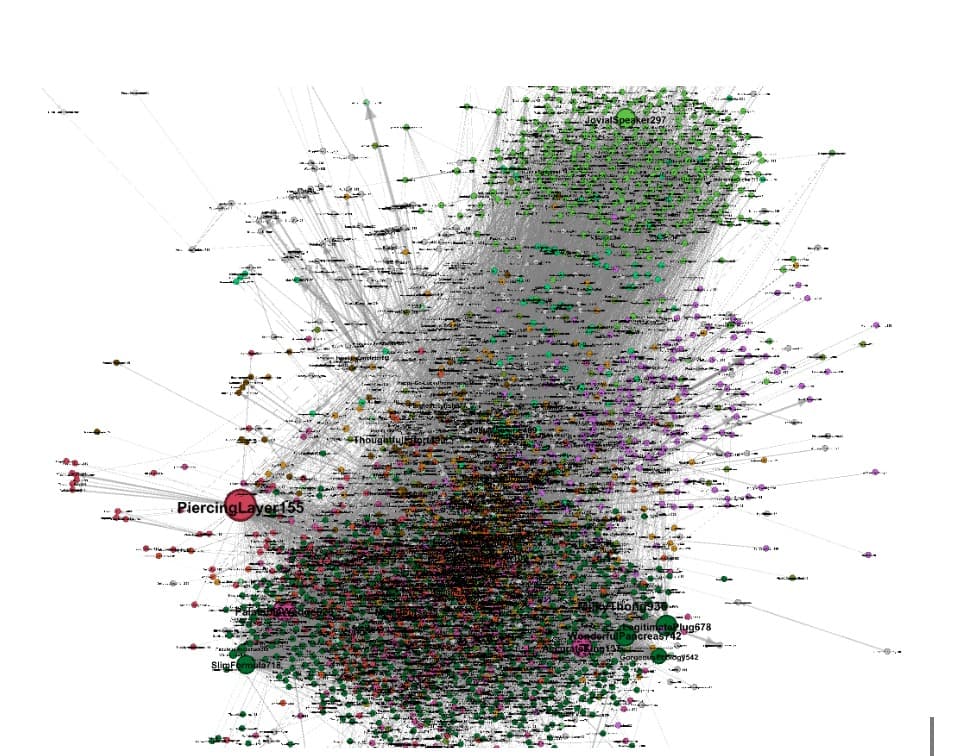
The detected communities mapped neatly onto recognisable shoe sub-cultures: a sneaker / streetwear cluster, a high-heels / fashion cluster, a fitness / running cluster, and a couple of smaller language-specific groups. That gave the brand a concrete second decision: a single influencer crossing communities, or several smaller-budget partnerships within each.

7. Information diffusion — an SIR sanity check

Centrality scores are static. They tell you a node's position, but not what would actually happen if it posted. To pressure-test the ranking, we ran an SIR (Susceptible–Infected–Recovered) diffusion simulation, treating "infection" as exposure to a sponsored post.

• Susceptible — has not seen the post yet.
• Infected — has seen the post and is reposting / sharing this round.
• Recovered — has seen the post but is no longer actively sharing.

For each candidate seed account from §5, we ran the SIR model many times and recorded the average final reach (total fraction of nodes that ever entered the I or R state).

import EoN  # or a small custom SIR loop
sim = EoN.fast_SIR(G_nx, tau=0.05, gamma=0.1, initial_infecteds=[seed])
final_reach = sim[3][-1] / G_nx.number_of_nodes()  # share of network reached

The PageRank top picks consistently produced larger final reach than the raw-followers top picks. That's the empirical version of the argument above — the structure-aware ranking doesn't just look better, it actually diffuses further under a simulated post.

8. Link prediction — who's about to connect

A small bonus analysis. Using common-neighbour and Jaccard-coefficient scores between non-adjacent pairs, we ranked likely future edges in the network. Two reasons to care:

1. If two communities are about to merge (lots of high-score pairs across their boundary), an influencer that's only top-ranked today might be less valuable than one positioned in the merging space.
2. The link-prediction scores are themselves a sanity check on the community detection — if predicted future edges fall mostly inside a detected community, the community is real; if they cross boundaries randomly, the partition is over-fitted.

preds = nx.jaccard_coefficient(G_nx.to_undirected())
top   = sorted(preds, key=lambda x: -x[2])[:50]

9. What I'd take into the next graph project

A few other things worth repeating:

• Reduce the network with structure, not at random. Random subsampling destroys the community signal you came to look for. Cluster first, keep the active parts.
• Always compute global metrics before running detection. Transitivity and reciprocity tell you whether community detection is even meaningful before you spend an hour on Louvain.
• Use two libraries. networkx for code that you'll read again later, igraph for anything that has to run on a graph with more than a few thousand nodes.
• Validate static rankings with a diffusion simulation. Centrality is structural; SIR is dynamic. They don't always agree, and when they don't, the dynamic answer is the one closer to what the brand will actually experience.

Resources