Before You Fix Your Data, Understand It.

Last update: April 2024. All opinions are my own.

Overview

Most Kaggle writeups start with "I trained XGBoost and tuned the parameters."
This one starts earlier -- with the part that actually saves time.

Forest Cover Type Prediction is a multiclass classification task: given cartographic variables, predict the forest cover type (classes 1-7) for each location.

The interesting part isn't the model. It's the features.

Many variables describe the same terrain from different angles (sometimes encoding the same signal), which means the highest-leverage step is understanding what the dataset is really measuring before you start "cleaning" or "optimizing".

TL;DR (what this post argues)

• Feature semantics beat hyperparameters early on.
• "Weird values" (zeros, negatives) often reflect geography, not bad data.
• Outliers in terrain datasets are frequently signal, especially when they cluster by class.

The mindset I used

• Interpret the feature: what does it mean physically?
• Validate suspicious patterns: zeros, negatives, skew
• Treat outliers as hypotheses: signal vs noise

That leads to three guiding questions:

• What do the cartographic features represent in real terrain?
• Are unusual values valid measurements or data issues?
• Are outliers noise -- or class-specific signal?

If you can answer those, model choice becomes easier, and a lot of "data cleaning" becomes unnecessary.

Dataset and Target

The dataset contains three feature groups:

• 10 numeric features
  (elevation, slope, distances to hydrology/roadways/fire points, hillshade variants)
• 4 one-hot wilderness area indicators
  (exactly one is active per row)
• 40 one-hot soil type indicators
  (exactly one is active per row)

The target is Cover_Type with 7 classes. The training set is relatively balanced, so accuracy is a reasonable first metric -- but per-class performance still matters to understand where cover types overlap.

The numeric features are far from Gaussian. Several distance features are long-tailed, and vertical distance to hydrology includes negative values -- valid, but easy to misread if you assume "distance must be positive".

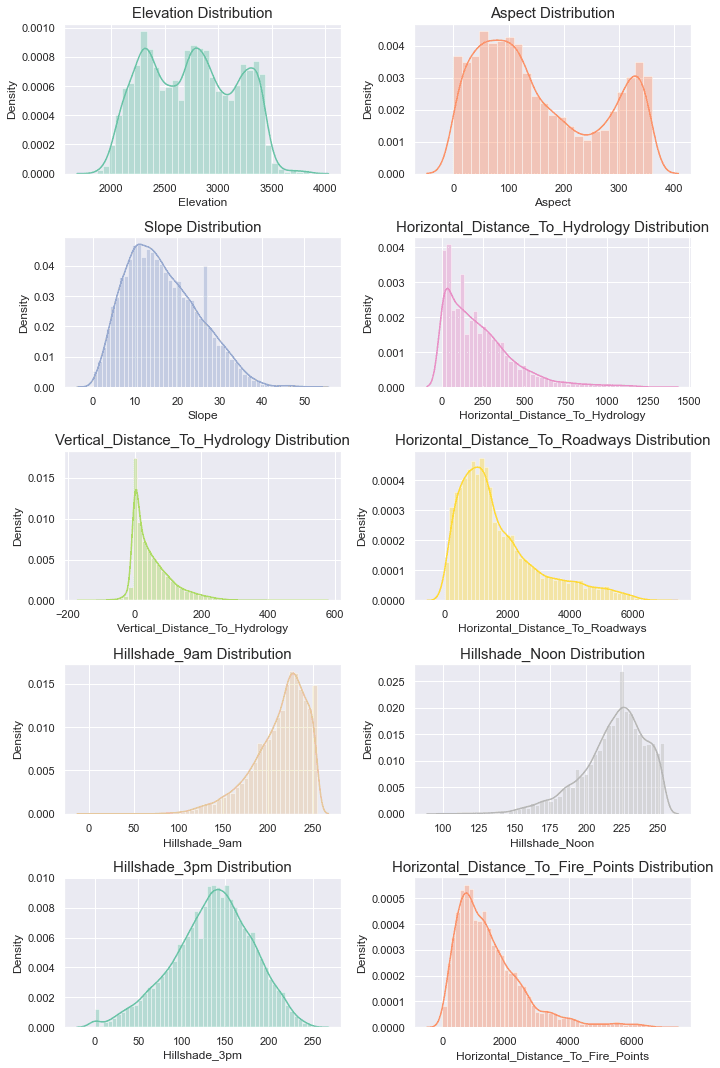
Note: In terrain datasets, "weird values" often mean geography, not bad data.

Feature Semantics

A useful mental model for this dataset:

• Some features are direct measurements (elevation, slope).
• Others are derived views of the same geometry (hillshade).
• Several distance variables encode similar structural information
  (proximity to hydrology, roads, fire points).

That redundancy can help tree ensembles -- but it can also:

• dominate distance metrics in KNN,
• inflate confidence if correlated features are treated as independent signal,
• encourage unnecessary "cleaning" when the patterns are actually valid.

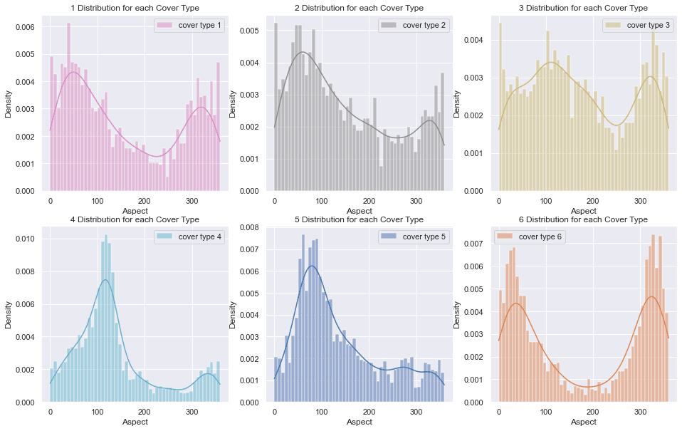
Terrain Geometry (Slope, Aspect, Hillshade)

• Slope captures steepness.
• Aspect captures direction/orientation (0-360 degrees).
• Hillshade captures illumination derived from slope + aspect + sun position (0-255).

Hillshade isn't "new information" in the same way elevation is -- it's a transformation of geometry. So I expect hillshade variants to correlate with aspect and with each other.

The correlation heatmap confirms that:

Tip: Aspect is a circular variable. For linear models, representing it as (sin(aspect), cos(aspect)) is often better than treating 0 and 360 as far apart. Tree models are usually fine with raw aspect.

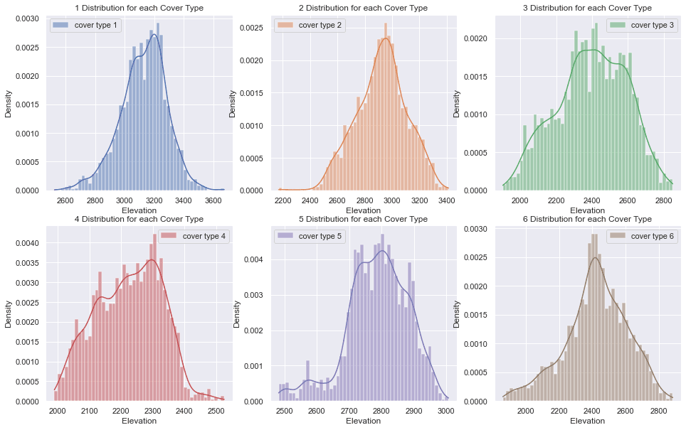
Elevation as a Primary Separator

Elevation is consistently a top discriminator in this dataset. The per-class elevation distributions show meaningful separation, which explains why elevation often dominates feature importance later.

If you only plot one feature, plot elevation.

Validating Weird Values (Instead of Automatically Cleaning)

Two patterns that are common "gotchas" here:

• Negative vertical distance to hydrology can mean the nearest water feature lies below the observation point. That is not an error.
• Hillshade_3pm = 0 can represent no illumination; if it appears frequently, it's worth validating rather than assuming corruption.

Instead of blindly replacing values, I tested whether these patterns were consistent with the rest of the terrain variables.

A small RandomForestRegressor worked well as a sanity check:
if hillshade is predictable from slope/aspect/elevation, then frequent zeros might be suspicious -- or reflect valid edge cases.

The goal was validation, not fixing.

from sklearn.ensemble import RandomForestRegressor
from sklearn.metrics import r2_score
from sklearn.model_selection import train_test_split

feature_cols = ["Elevation", "Slope", "Aspect", "Hillshade_9am", "Hillshade_Noon"]
target_col = "Hillshade_3pm"

X = df[feature_cols]
y = df[target_col]

X_train, X_val, y_train, y_val = train_test_split(
    X, y, test_size=0.2, random_state=42
)

model = RandomForestRegressor(
    n_estimators=200,
    random_state=42,
    n_jobs=-1,
)
model.fit(X_train, y_train)
preds = model.predict(X_val)

print("R2:", r2_score(y_val, preds))

Result: Hillshade was highly predictable from slope/aspect/elevation, which suggests frequent zeros are more likely valid lighting edge cases than data corruption.

Workflow

The project followed a disciplined sequence:

1. Validate the dataset and feature constraints.
2. Understand distributions and suspicious values.
3. Establish baselines (to set expectations and catch mistakes).
4. Train stronger models only after the data makes sense.

Data Checks

These checks are boring - and that's why they work.

• Verified feature types and ranges.
• Confirmed one-hot groups sum to exactly one per row.
• Checked class balance.
• Reviewed numerical distributions and scaling needs.

A quick sanity check for the one-hot groups:

wilderness_cols = [c for c in df.columns if c.startswith("Wilderness_Area")]
soil_cols = [c for c in df.columns if c.startswith("Soil_Type")]

assert (df[wilderness_cols].sum(axis=1) == 1).all()
assert (df[soil_cols].sum(axis=1) == 1).all()

That single assertion prevents a surprising number of downstream "mystery bugs."

Evaluation Setup

I used a stratified train/validation split and tracked both accuracy and macro F1. Accuracy is fine for a balanced dataset, but macro F1 surfaces the cover types that overlap most.

Pitfalls to avoid: Scale numeric features for KNN/logistic regression, treat aspect as circular for linear models, and remember that "distance" includes both horizontal and vertical components.

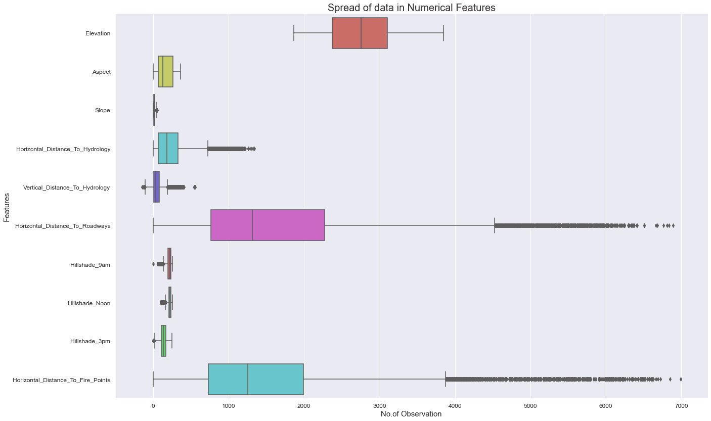
Outlier Analysis

With terrain data, outliers are rarely random. They usually reflect something real in the geography:

• rare geographic regimes (high elevation zones, unusual terrain)
• extreme slopes or ridges
• edge cases that genuinely belong to specific cover types

Because the numerical features are skewed (and several distance features are long-tailed), I used a conservative 3xIQR rule to flag extreme values - then asked the more important question:

Do these outliers behave like noise, or do they cluster by cover type?

What I Found

• Outliers were not evenly distributed across classes.
• Many outliers were concentrated in specific cover types.
• Removing them did not improve validation performance, so I kept them.

In other words: in this dataset, outliers often behave like signal, not corruption.

Boxplots made the long tails and extreme values easy to interpret, especially for distance features:

Computing the Outlier Mask

q1 = df[numeric_cols].quantile(0.25)
q3 = df[numeric_cols].quantile(0.75)
iqr = q3 - q1

outlier_mask = (df[numeric_cols] < (q1 - 3 * iqr)) | (df[numeric_cols] > (q3 + 3 * iqr))

Rule of thumb: If outliers cluster by class, they are usually worth keeping - they often represent meaningful terrain regimes rather than noise.

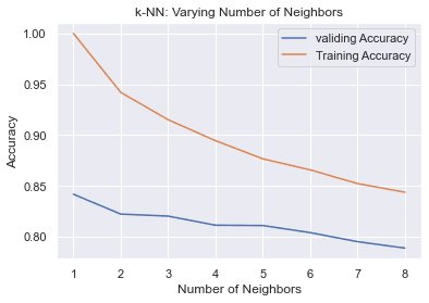
Baseline Models

Before using heavier models, I started with lightweight baselines for two reasons:

1. Establish a reference level of performance
2. Catch pipeline mistakes early (encoding, scaling, leakage)

Baselines:

• Naive Bayes
• KNN
• Logistic Regression

KNN served as a useful "geometry sanity check" because it reflects local structure in feature space. Validation accuracy peaked at small k and degraded as k increased, consistent with meaningful local neighborhoods.

Feature Engineering and Dimensionality Reduction

Given redundancy between terrain variables, I explored feature selection and PCA mainly as ways to:

• reduce correlated dimensions,
• stabilize some learners,
• understand whether variance concentrates in a smaller subspace.

Two practical notes:

• PCA is most meaningful on continuous terrain variables (hillshade + distances + elevation/slope).
• Applying PCA over one-hot soil indicators is usually less interpretable; tree models handle them better directly.

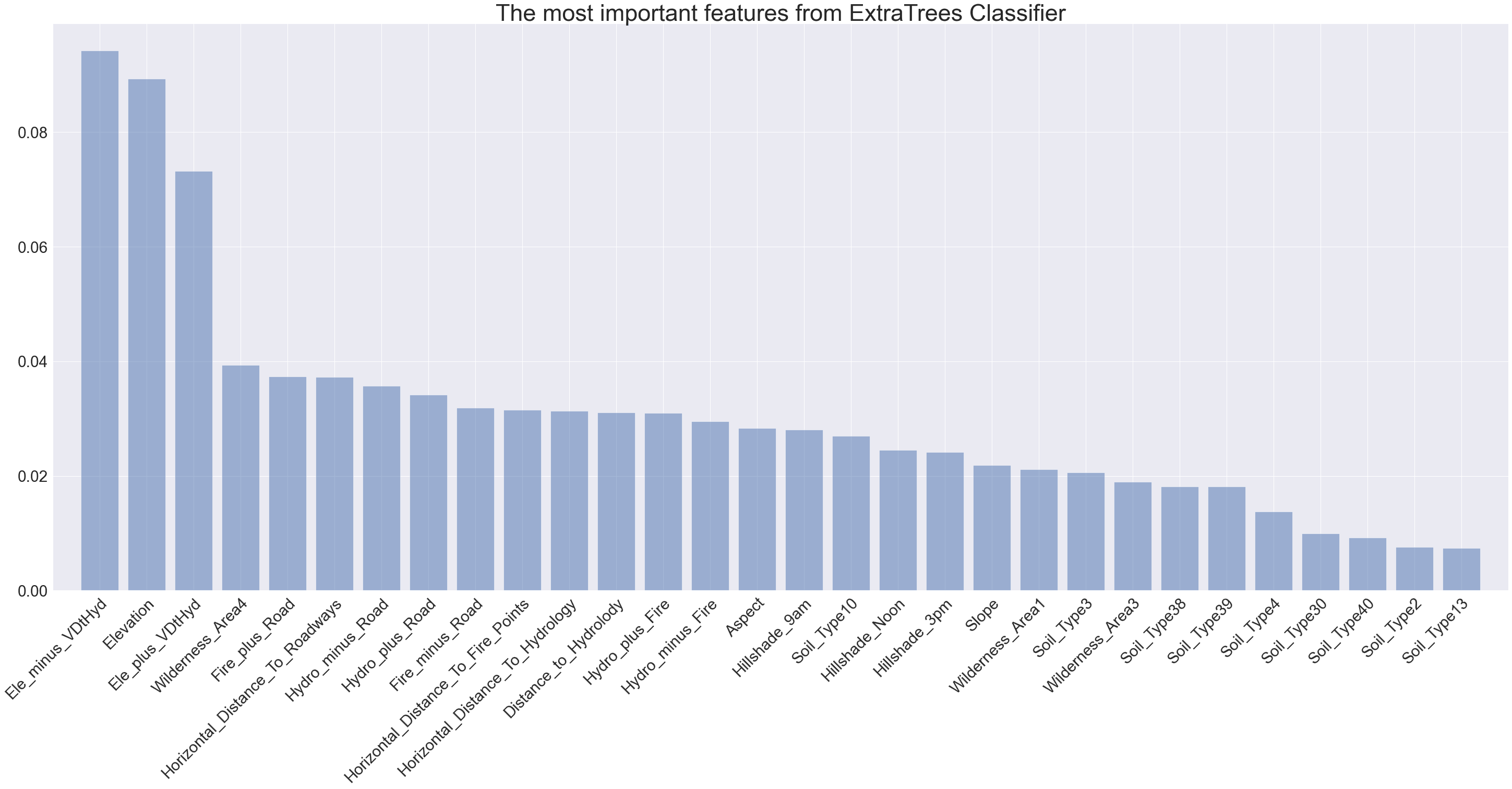
Stronger Models and Tuning

Once the data checks and baselines looked sane, I moved to tree-based ensembles. They performed best because they naturally capture:

• non-linear interactions (elevation x slope, soil x wilderness)
• threshold effects common in terrain systems
• redundancy without needing explicit de-correlation

Models explored:

• Gradient Boosting
• Random Forest
• Extra Trees
• Hyperparameter tuning to improve generalization

Results and Key Takeaways

The final pipeline achieved strong accuracy, but the most valuable lessons were not about the model - they were about the dataset.

• Elevation is the strongest discriminator across cover types.
• Outliers can be useful signal, especially when they cluster by class.
• Some terrain features encode redundant information (hillshade vs aspect/slope).
• The highest leverage step was validating what the dataset actually measures.

Feature importance echoed the EDA: elevation and hydrology-related distances dominate, while hillshade and soil indicators add finer-grained separation.

If I had to summarize the project in one sentence:

The model becomes easier when the data stops being a mystery.

Next Steps

If I continued improving this project, these are the next steps I'd prioritize:

• Represent aspect as sin/cos for linear models (better circular handling).
• Apply log transforms to long-tailed distance features.
• Use confusion matrices and per-class metrics to see where cover types overlap.
• Add calibration if probability estimates matter.
• Run error analysis by terrain regime (high elevation vs low elevation subsets).

These steps are not "Kaggle tricks" - they translate directly to real ML work.

Skills and Tools

• Python
• Matplotlib, Seaborn, Plotly
• scikit-learn pipelines
• Feature engineering and preprocessing
• Model comparison and hyperparameter tuning

Resources

If you want to explore the full notebook or reproduce the workflow:

• Kaggle competition: Forest Cover Type Prediction
• UCI Covertype dataset
• ArcGIS: how hillshade works

• Notebook (Jupyter)

• GitHub Repository

• Run on Colab