Three Ways to Encode an Hour of the Day

Last update: January 2024. All opinions are my own.

A team project (Group A, IE MBD, January 2024) forecasting hourly bicycle demand for the Washington, D.C. bike-share system. The interesting part isn't the model — it's how you encode time. Hour-of-day, day-of-week, and month-of-year are all cyclic, and treating them as plain integers wastes the structure.

1. The dataset

The dataset is a row per hour of operation between 2011 and 2012, with weather, calendar, and rider counts. The target is cnt — total rentals that hour.

2. EDA — the things you only see if you look

2.1 An October 2012 outage hiding in plain sight

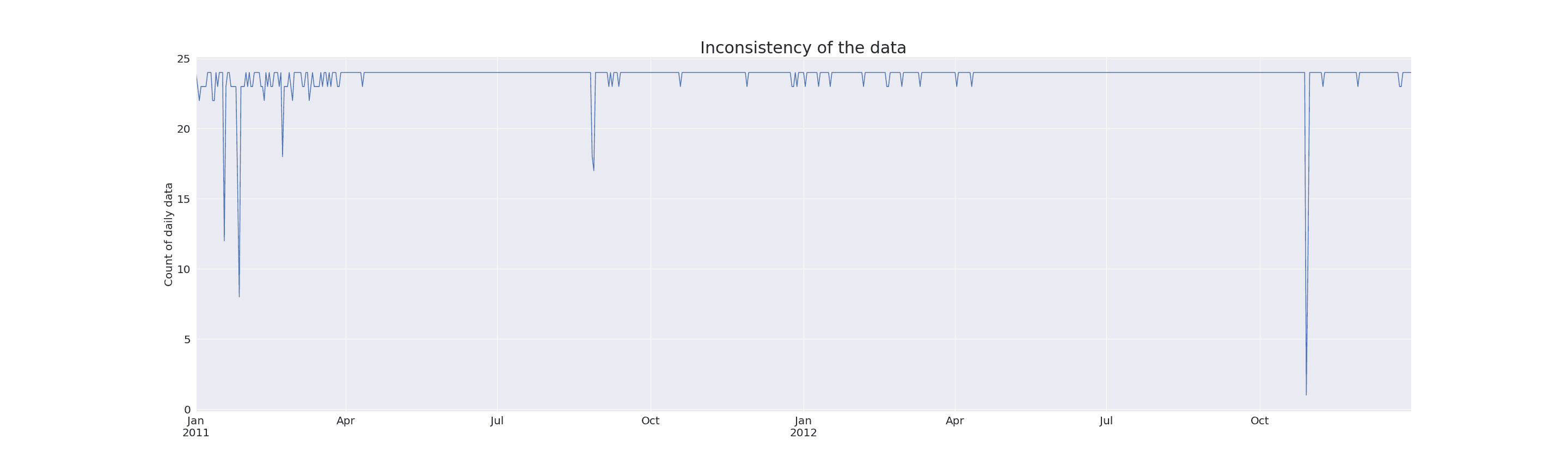
A simple plot of hourly demand over time revealed something weird: a 23-hour gap in October 2012 where the system reported essentially zero rentals. Not noise — a real outage. Worth catching before treating the data as a clean time series.

2.2 Skewness in windspeed

Most numerical features had reasonable distributions, but windspeed was strongly right-skewed — long tail of high values. Applying a log1p transform pulled it into a much more usable shape and reduced its outlier influence.

2.3 The shape of the day

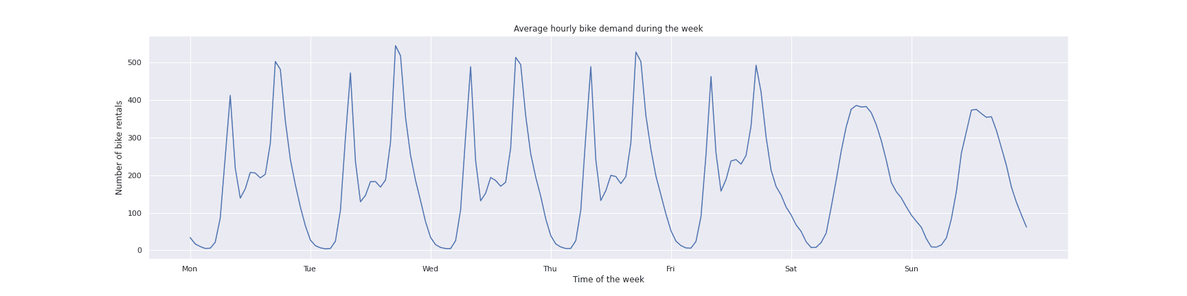
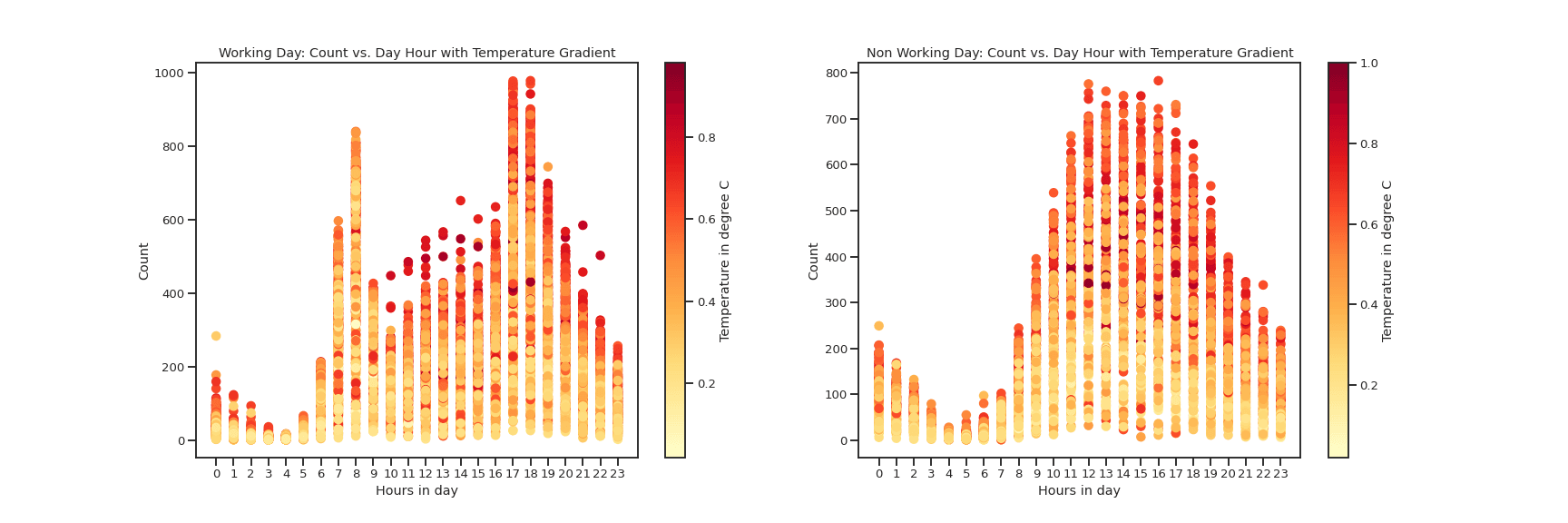
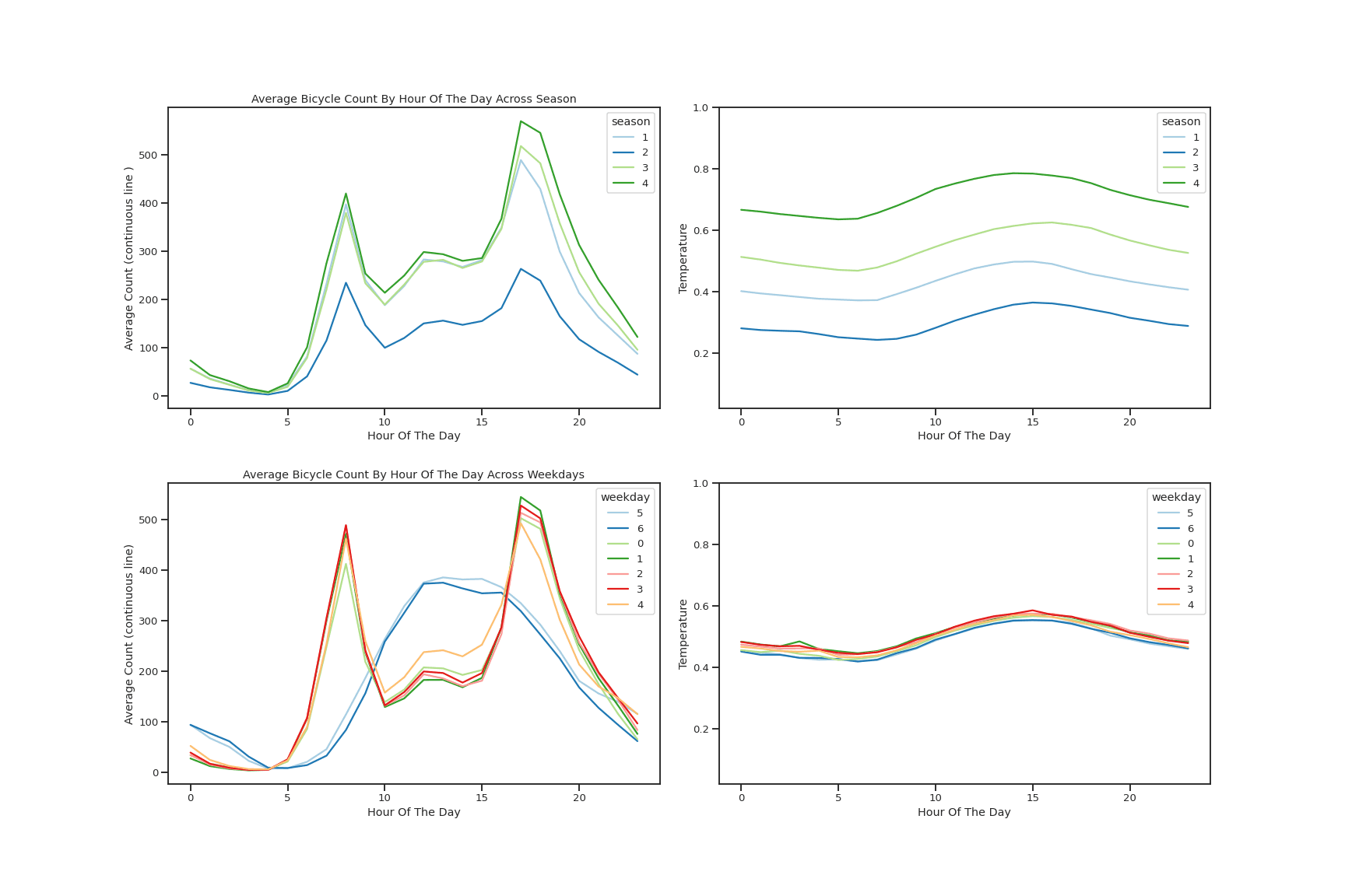
The hourly demand pattern is bimodal on working days — a tall morning rush around 8 AM and an even taller evening rush around 5 PM. Weekends are completely different: a single afternoon hump and no rush hours at all.

2.4 Season and weather

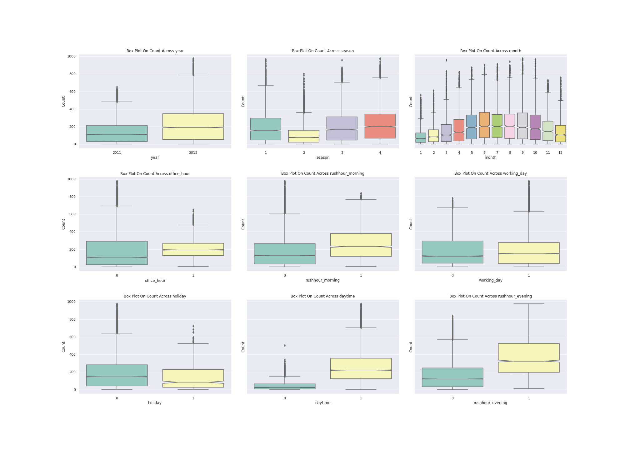
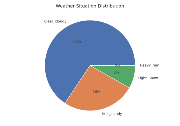
Seasonal pattern is exactly what you'd expect: highest demand in summer and fall, lowest in winter. Bad weather flattens the day.

3. Time-based cross-validation — no random splits

The single biggest mistake in time series forecasting is using a random train/test split. It leaks the future into the past — the model "sees" tomorrow when it shouldn't.

For this dataset, the train/test boundary was September 30, 2012, with the test set being the last quarter of 2012. Inside training, we used TimeSeriesSplit with a 2-day gap between train and test segments and a fixed 1000-point test window per fold (roughly 6 weeks — enough to span weekly cycles).

train = df.loc[df['dteday'].isin(pd.date_range(start='01/01/2011', end='30/09/2012'))]
test  = df.loc[~df['dteday'].isin(pd.date_range(start='01/01/2011', end='30/09/2012'))]

4. The three ways to encode time

Hour-of-day, day-of-week, and month-of-year are cyclic: hour 23 is closer to hour 0 than to hour 12, but a plain integer encoding can't express that. So we built three different ColumnTransformer pipelines and let them race.

4.1 Transformer 1 — time as raw numerical features

The simplest. Treat hr, weekday, month, etc. as continuous variables and scale them with MinMax. Cheap, but the model has to learn the cyclical structure from scratch.

transformer = make_column_transformer(
    ('drop', ['atemp', 'dteday', 'casual', 'registered']),
    (KNNImputer(n_neighbors=2), ['temp']),
    (SimpleImputer(strategy='median'), ['hum']),
    (SimpleImputer(strategy='median'), ['windspeed']),
    (make_pipeline(SimpleImputer(strategy='most_frequent'),
                   OneHotEncoder(handle_unknown='ignore')), ['weathersit']),
    remainder=MinMaxScaler(),
)

4.2 Transformer 2 — one-hot encode every time feature

Treat hr, weekday, month, season, etc. as categorical and one-hot encode all of them. The model gets a separate degree of freedom for every hour-of-day, every weekday, every month. Very flexible, but explodes the feature count and ignores the ordering of the values.

time_related_features = [
    'season', 'month', 'year', 'weekday', 'working_day',
    'office_hour', 'daytime', 'rushhour_morning', 'rushhour_evening',
    'highseason', 'holiday', 'hr',
]

one_hot_transformer = make_column_transformer(
    ('drop', ['atemp', 'dteday', 'casual', 'registered']),
    (KNNImputer(n_neighbors=2), ['temp']),
    (SimpleImputer(strategy='median'), ['hum']),
    (SimpleImputer(strategy='median'), ['windspeed']),
    (make_pipeline(SimpleImputer(strategy='most_frequent'),
                   OneHotEncoder(handle_unknown='ignore')), ['weathersit']),
    (OneHotEncoder(handle_unknown='ignore'), time_related_features),
    remainder=MinMaxScaler(),
)

4.3 Transformer 3 — cyclic features via sin/cos

This is the interesting one. Replace each cyclic integer with a (sin, cos) pair on a circle:

def sin_transformer(period):
    return FunctionTransformer(lambda x: np.sin(x / period * 2 * np.pi))

def cos_transformer(period):
    return FunctionTransformer(lambda x: np.cos(x / period * 2 * np.pi))

cyclic_transformer = make_column_transformer(
    ('drop', ['atemp', 'dteday', 'casual', 'registered']),
    (KNNImputer(n_neighbors=2), ['temp']),
    (SimpleImputer(strategy='median'), ['hum']),
    (SimpleImputer(strategy='median'), ['windspeed']),
    (make_pipeline(SimpleImputer(strategy='most_frequent'),
                   OneHotEncoder(handle_unknown='ignore')), ['weathersit']),
    (sin_transformer(12), ['month']),  (cos_transformer(12), ['month']),
    (sin_transformer(7),  ['weekday']),(cos_transformer(7),  ['weekday']),
    (sin_transformer(24), ['hr']),    (cos_transformer(24), ['hr']),
    remainder=MinMaxScaler(),
)

The sin/cos pair encodes the angle of the hour on a 24-hour clock. Same trick works for weekday (period 7) and month (period 12). It costs 2 features per cyclic variable — much less than the one-hot blow-up.

5. The three models

For each transformer, we tried three models:

pipelines = {
    'Linear Regression':  Pipeline([('t', transformer), ('m', LinearRegression())]),
    'Random Forest':      Pipeline([('t', transformer), ('m', RandomForestRegressor())]),
    'Decision Tree':      Pipeline([('t', transformer), ('m', DecisionTreeRegressor())]),
}

That's 3 transformers × 3 models = 9 configurations to evaluate.

6. Grid search + time-aware CV

Each pipeline went through a grid search over its hyperparameters, evaluated with TimeSeriesSplit cross-validation. The 1000-point window with a 2-day gap kept the validation realistic: the model only ever saw the past at training time.

The winning configuration ended up being Transformer 1 (numerical time features) paired with the best-tuned Random Forest from grid search. The intuition: tree-based models can find non-linear splits on hr directly, so they don't need the cyclic structure encoded explicitly — and they avoid the dimensionality blow-up of the one-hot variant.

For linear models the ranking was different: the cyclic transformer was a clear win over numerical, since linear regression really cannot express "hour 0 is close to hour 23" without help.

7. What I'd take into the next time series

A few other things worth repeating:

• Plot demand over time before doing anything else. The October 2012 outage was invisible in aggregate statistics — only the time-of-day chart caught it.
• Use TimeSeriesSplit with a gap. Random KFold on time-ordered data leaks the future into the validation score and you get a model that looks great in development and fails on day one.
• Tree-based models are happy with numerical time features. Save the one-hot/cyclic encodings for linear models, where the encoding is doing real work.
• Always look at predicted-vs-actual on the held-out period. A model that does well on cross-validation but visibly misses rush hour is hiding something the score isn't telling you.

Related Kaggle write-ups

Two more from the same family — each one starts with feature semantics before any model:

• Before You Fix Your Data, Understand It (Forest Cover Type) — cartographic features, sanity checks, and why "weird values" often mean geography rather than bad data.
• When Missing Values Aren't Random (Spaceship Titanic) — relational imputation from PassengerID and Cabin schemas, plus a 10-model bake-off.

Resources