
Table of Contents
- 1. What AWS DeepRacer actually is
- 2. The architecture behind training
- 3. The reward function — how the car learns what "good" means
- 4. The parameters you have to work with
- 5. The reward function I actually shipped
- 6. Hyperparameters that actually matter
- 7. PPO vs SAC — choosing the algorithm
- 8. Action space and calibration
- 9. ROS — how the agent talks to the environment
- 10. Moving from simulator to a real track
- 11. What I'd do differently next time
Last update: October 2023. All opinions are my own.
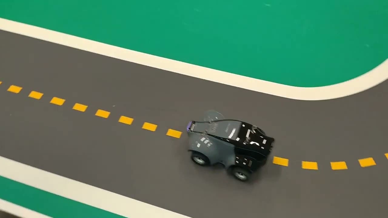
For a few weeks during my MSc, I had a 1/18-scale toy car learning to drive itself around a virtual racetrack. The car is AWS DeepRacer — Amazon's reinforcement-learning playground — and the single most important thing I learned is this:
The bug is always in the reward function, never in the agent.
My first model drove perfectly centred down every straight and crawled around every corner. I thought it was broken. It wasn't — it was an A-student. I'd written a reward function that paid out for "stay near the centre" and nothing else, and the agent did precisely that. The model was a star pupil; I was a bad teacher.
This post is what I learned trying to be a better one — the cloud architecture behind training, every parameter you can use in a reward function, the hyperparameters worth tuning, and the gap between simulator and a real track.
What AWS DeepRacer actually is
AWS DeepRacer is a 1/18-scale autonomous car you train with reinforcement learning. You write a Python reward function, pick a few hyperparameters, and a model trains in the cloud against a simulated track. Once it's good in the simulator, you can deploy it onto a physical car on a real track.
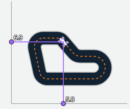
The track I worked on is the Cumulo Turnpike — 60 m × 106 cm, a layout that punishes anyone who can't take corners cleanly. To make the car faster you need a better RL model, which means more iteration on the reward function and a smarter choice of hyperparameters.
The architecture behind training
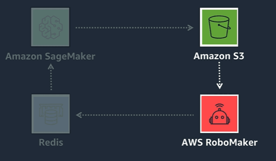
DeepRacer training is split across five AWS services that talk to each other in a loop. SageMaker runs the RL algorithm and updates the neural network. RoboMaker hosts the simulator and runs the agent (the car) inside it, using Gazebo as the physics engine — chassis, wheels, camera, friction, collisions, accelerations. Amazon S3 stores the persisted copy of the model, and Redis is the in-memory database that caches every (state, action, reward, next-state) tuple produced by the agent.
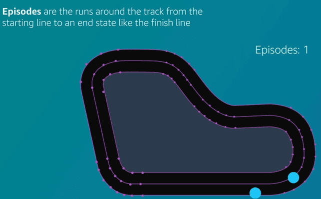
Each episode is a full run from the starting line to the finish line (or until the agent leaves the track). Each episode is broken into steps. For every step, the (state, action, reward, next state) tuple is stored in Redis and used to update the policy network in SageMaker.
The reward function — how the car learns what "good" means
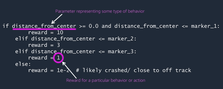
In ML you have parameters (learnable weights) and hyperparameters (you set them). In RL you have a third thing: a reward function. Each step, the simulator passes the function a dictionary of state variables and the function returns a number — the reward for that step. Bigger reward = "more like this."
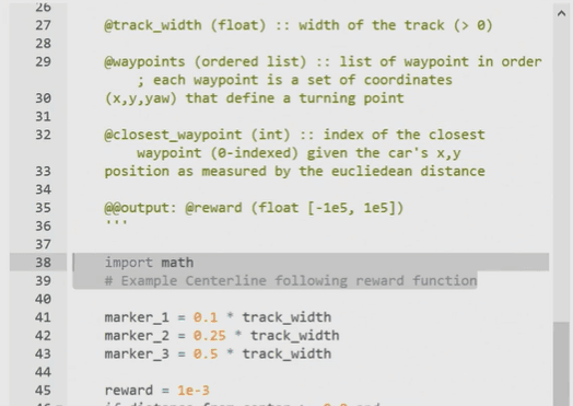
The canonical starter reward function uses three distance markers from the centre line:
def reward_function(params):
    track_width = params['track_width']
    distance_from_center = params['distance_from_center']

    marker_1 = 0.1 * track_width
    marker_2 = 0.25 * track_width
    marker_3 = 0.5 * track_width

    if distance_from_center <= marker_1:
        return 1.0          # right in the middle — great
    elif distance_from_center <= marker_2:
        return 0.5          # off-centre but ok
    elif distance_from_center <= marker_3:
        return 0.1          # near the edge
    else:
        return 1e-3         # likely crashed or off-track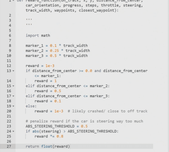
The reward function is the single most important thing you write.
The model can only optimise for what you reward. Reward "stay in the centre" and you get a slow, perfectly-centred car. Reward "go fast and stay on the track" and you get something more interesting — but you also have to balance the two carefully so it doesn't learn to spin out at the first corner.
The parameters you have to work with
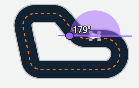
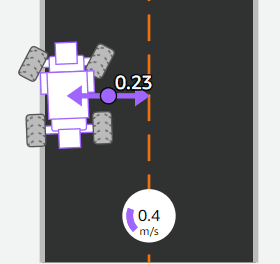
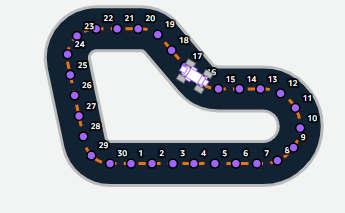
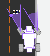
The state dictionary passed into the reward function has more than twenty fields. They're the entire vocabulary you can use to describe "what's happening right now." The figure below is the one I came back to most often — it shows the main spatial parameters laid out on a single car-on-track illustration.
The ones I reached for most:
- distance_from_center +
track_width— the "stay centred" signal. - all_wheels_on_track — boolean; useful as a hard penalty (or a hard zero).
- progress +
steps— the most underrated combination. Progress / steps is a proxy for speed, and rewarding it directly teaches the car to finish laps faster instead of just driving carefully. - waypoints +
closest_waypoints— when you want to nudge the car toward a racing line rather than the geometric centre.
The reward function I actually shipped
After working through the parameter reference, my final reward function ended up using just three of the available signals: a hard gate on staying on the track, a measure of efficiency (progress per step), and a direct speed bonus.
def reward_function(params):
    if params['all_wheels_on_track'] and params['steps'] > 0:
        reward = (params['progress'] / params['steps']) * 100
        reward += params['speed'] ** 2
    else:
        reward = 0.01
    return float(reward)
The all_wheels_on_track gate gives near-zero reward (0.01) the moment any wheel leaves the track — the agent learns to treat the borders as a wall. The progress / steps term rewards efficient lap completion — a tighter line covers more track per decision. And speed² pushes the throttle harder: the squaring means the difference between 4 m/s and 5 m/s (the action-space ceiling) is worth a lot more than the difference between 1 m/s and 2 m/s.
Constraining myself to three signals made the reward easy to reason about. When the agent did something weird, I could point at one of three terms — not a tangle of competing incentives.
Hyperparameters that actually matter
You can't learn hyperparameters from the data — you set them, then iterate. DeepRacer exposes eight of them through the console.
Batch size
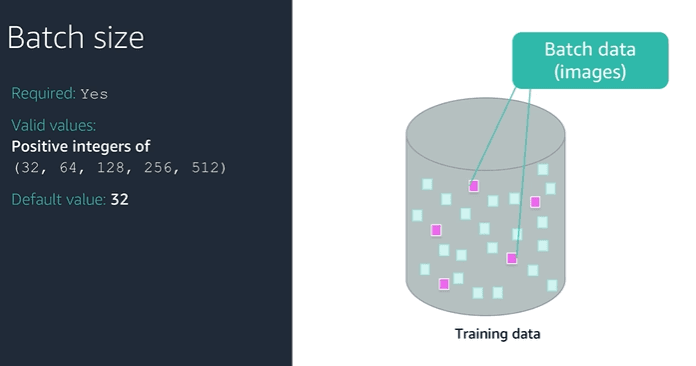
How many samples the model processes before each weight update. Bigger batches give smoother gradients but slower iteration. Defaults to 32; I had better luck with 64 once the reward function stopped changing.
Number of epochs
How many passes the trainer makes over each batch before updating. Larger numbers help when the batch size is big. Too many and the model overfits to recent experience.
Learning rate
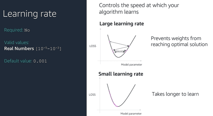
The single biggest tuning lever. Too large and weights overshoot the optimum; too small and the model is still mediocre when your AWS credits run out.
Exploration
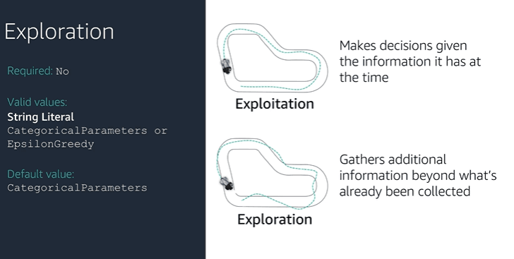
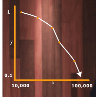
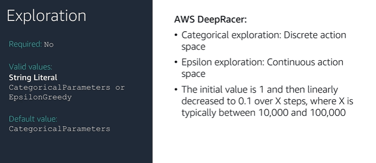
The policy either uses Categorical sampling (sample an action from the policy's probability distribution) or Epsilon-greedy (take the best action most of the time, but a random one with probability ε that decays from 1 → 0.1 over training).
Exploration vs exploitation is the central tension. Exploitation = use what you already know works. Exploration = try things you haven't and see if they lead somewhere better. Tune this badly and the car either gets stuck in a local optimum (too much exploitation) or never converges (too much exploration).
Entropy
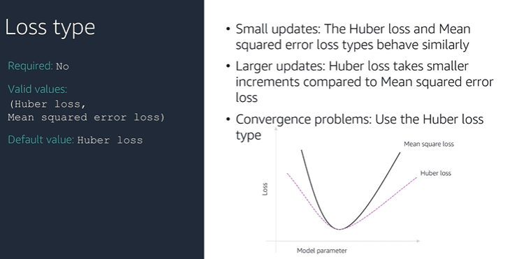
Default 0.5. Higher entropy keeps the agent exploring within its current policy; lower entropy makes it confidently exploit what it has learned. Too high and the agent never converges; too low and it gets stuck in suboptimal patterns.
Discount factor
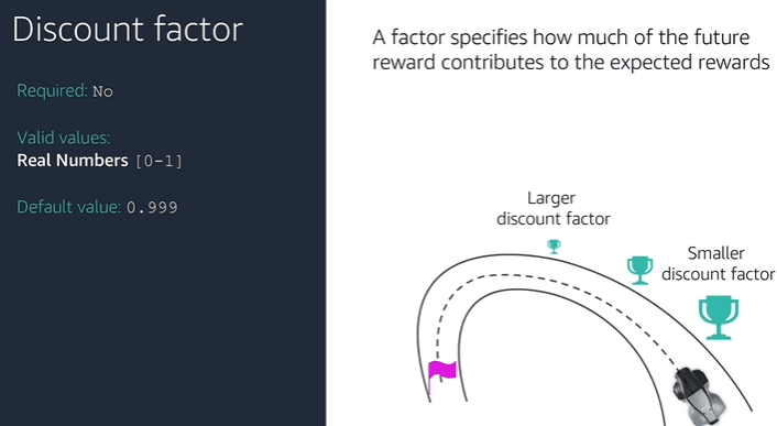
Default 0.999. How much future rewards count relative to immediate ones. 0.999 is unusually high; if your reward function is per-step (like mine), a lower factor often helps because the agent doesn't need to plan as far ahead.
Loss type
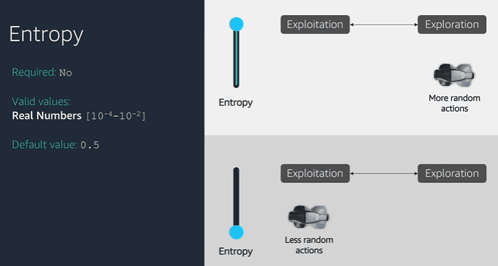
Default Huber. Huber takes smaller increments than MSE on big errors, which makes it more stable when convergence is hard. Use MSE if convergence is fine and you want to train faster.
Number of episodes
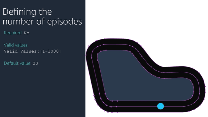
More episodes means more experience to learn from — and more training time and credits. Cap your budget here.
PPO vs SAC — choosing the algorithm
DeepRacer lets you train with two algorithms: PPO (Proximal Policy Optimization) and SAC (Soft Actor-Critic). PPO is the default and works well as a first pass.
PPO works with both discrete and continuous action spaces. SAC only works with continuous ones — so if you're using the default 6-action discrete space (Straight, Shallow/Deep Left, Shallow/Deep Right, Slow), PPO is decided for you.
PPO is on-policy: it only learns from experiences generated by its current policy. SAC is off-policy: it can reuse experiences from past policies, which makes it more data-efficient at the cost of stability. On-policy methods are smoother between iterations; off-policy methods can lose their grip mid-training when very different past experiences get mixed in.
A policy with low entropy is very confident about its action; a high-entropy policy is unsure. SAC explicitly rewards uncertainty, which keeps the agent exploring even late in training. The SAC alpha hyperparameter controls the trade-off — at the maximum, the policy is all entropy and forgets to maximise reward; at the minimum, it collapses to standard RL with no exploration bonus. A starting point of 0.5 is reasonable; iterate from there.
Action space and calibration
The action space defines every possible move the agent can make. DeepRacer's default discrete action space has six options:
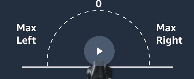
Each action combines a throttle value and a steering angle: Straight, Shallow Left, Deep Left, Shallow Right, Deep Right, and Slow. When you calibrate the physical car, you set the throttle and steering bounds — and those bounds need to match the simulator's action space, otherwise sim-to-real transfer breaks.
Faster speeds take longer to train. Models with higher maximum speeds take more episodes to converge than slower ones, because the agent has to learn to handle higher-momentum mistakes.
ROS — how the agent talks to the environment
So SageMaker trains the model, RoboMaker simulates the environment, Gazebo runs the physics. How do these actually communicate? Through ROS — the Robot Operating System. ROS is a set of libraries and tools that lets the components of a robot pass messages to each other: the camera publishes images, the policy node subscribes to them and publishes a steering command, the motor controllers subscribe to that and turn the wheels.
Once you move from simulator to a real car, the same ROS nodes do the inference. The only thing that changes is where the camera images and motor commands come from.
Moving from simulator to a real track
This is the genuinely hard part. The simulator can't reproduce everything about the real world — gravity, variable surface friction, lighting, motor calibration. So your beautiful sim lap becomes a confused real-car that drifts and stops at random.
There are three strategies to bridge that gap.
1. Environment control
The simulator tries to be representative of what the real world looks like — sky, grass, dark road — and the physics maps simulator actions to outcomes that closely match the real car. Throttle at 40% in the simulator should mean roughly the same wheel speed at 40% throttle on the physical car.
2. Domain randomisation
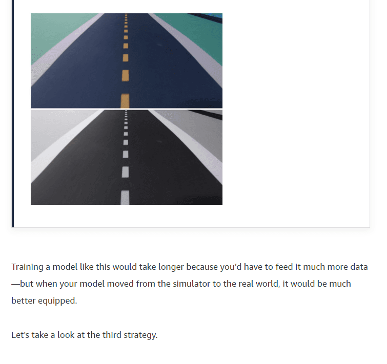
The camera images get converted to greyscale before they hit the model — so the model learns to track the dividing line, not "the colour white on the colour black." But if your real-world track has a yellow line instead, the model is confused. Domain randomisation deliberately randomises colours, textures and lighting in the simulator during training. The model learns to ignore those features and focus on the geometry, which transfers much better.
3. Modularity and abstraction
Pre-train a CNN on classifying generic visual concepts — "road", "not road", "line", "car", "building" — then plug that classifier in as a feature extractor before your RL model. The reasoning is that visual understanding is reusable. A CNN that already knows what a road is can teach an RL model faster than starting from raw pixels.
What I'd do differently next time
The single biggest mistake on my first model was rewarding "stay in the centre" too aggressively. The car learned to drive perfectly centred — and slowly. Adding a progress / steps term to the reward function (basically, "how much track did you cover per step?") was what made it competitive.
A few other things I'd keep in mind from the start:
- Start with PPO and the default hyperparameters. Get a model that finishes a lap. Then iterate.
- Don't tune more than one hyperparameter at a time. You will get confused about what helped.
- Look at the training graphs after every iteration. If the reward is going up but the lap completion rate isn't, your reward function is rewarding the wrong thing.
- Budget at least an hour of training per non-trivial change. The car is learning a continuous policy from sparse rewards — that takes time.